
7 What a Neural Network Can and Cannot Fit
7.1 Simple neural networks
We want to understand the fitting capabilities of neural networks built from layers with just one neuron, and compare them to a network with one wide hidden layer. Use PyTorch to build and fit the networks,1Another framework is fine if you prefer it. Do not write the backpropagation yourself: the point here is the comparison between architectures, not the derivatives, and PyTorch computes these with automatic differentiation. and use a GPT as your programming assistant. Your job is to decide what to measure, to check that the numbers are believable, and to explain what you see.
The reference numbers in the tables below come from a run of our own. Yours will differ in the last digits, because the data and the initial parameters are random. If they differ in the first digit, something is wrong.
7.1.1 The data
Take the function \[ f(x) = e^{-(x-3)^2/8}, \] a bump centred at \(x=3\), and observe it with noise, \[ y = f(x) + \varepsilon, \qquad \varepsilon\sim U[-0.1, 0.1]. \] Draw \(400\) training points with \(x\sim U[-5,11]\) and another \(400\) test points the same way. Two numbers are worth computing before you fit anything: the variance of the noise, \(0.2^2/12 \approx 0.0033\), and the variance of \(f(x)\) over the sample, \(\approx 0.125\).
The first is the noise floor: no model can do better than a mean squared error of \(0.0033\) on fresh data, because that part of \(y\) is not a function of \(x\). The second is what a model achieves when it predicts a constant: it explains nothing at all. Every MSE you report should be read against these two numbers.
Since \(x\) ranges over \([-5,11]\), it helps to standardize it, i.e. to feed \((x-\bar x)/s\) to the network rather than \(x\) itself, where \(\bar x\) and \(s\) are the mean and standard deviation of the training inputs.
7.1.2 Stacking single neurons
Build a network of \(L\) hidden layers with exactly one neuron per layer, and one output neuron: \[ z_i = a_i h_{i-1} + b_i, \quad h_i = \tanh(z_i), \quad i=1,\ldots,L, \qquad \hat y = a_{L+1}h_L + b_{L+1}. \] So every hidden layer uses \(\tanh\) as its activation function, and the output neuron uses the identity: we are predicting a number, not a probability, so there is no \(\sigma\) at the end. Train with the squared-error loss and mini-batch gradient descent.
Exercise 1.
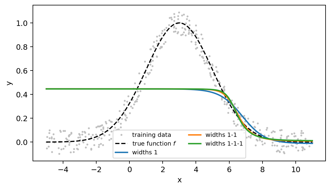
Fit this network for \(L=1,2,3\). Report the training and test MSE, and plot the fitted curve on top of the data. Since the training risk is not convex, fit each architecture from a few random initializations and keep the best one; otherwise you may be reporting a bad local minimum instead of a property of the architecture.
Solution
With \(400\) training points, batches of \(32\), learning rate \(0.1\), \(1500\) epochs and the best of \(3\) initializations, we obtained
| widths | parameters | train MSE | test MSE |
|---|---|---|---|
| 1 | 4 | 0.09534 | 0.09643 |
| 1-1 | 6 | 0.09424 | 0.09517 |
| 1-1-1 | 8 | 0.09416 | 0.09507 |
Against the noise floor of \(0.0033\) these are all bad, and adding layers barely changes anything: the third layer improves the training MSE from \(0.09534\) to \(0.09416\). The fitted curve is a descending step. It is flat at about \(0.45\) to the left of the bump and drops to \(0\) to the right of it.
Exercise 2.
Adding layers does not help here, and the reason is not that gradient descent got stuck. Prove that a network with one neuron per layer can never fit this data well, whatever its depth and whatever its parameters.
Hint: what kind of function is \(x\mapsto\tanh(ax+b)\), and what happens when you compose two such functions?
Solution
Each map \(t\mapsto \tanh(a t + b)\) is monotone: increasing if \(a>0\), decreasing if \(a<0\), since \(\tanh\) is increasing. A composition of monotone functions is again monotone, and so is the final affine step. Hence the network output is a monotone function of \(x\) for every choice of parameters and for every depth \(L\). The bump \(f\) increases up to \(x=3\) and decreases after it, so no monotone function can follow it. The best a monotone fit can do is something like the step we found.
This is a statement about the model class \(\Fset\), not about the optimizer. The same argument works for the sigmoid and for the ReLU, since both are non-decreasing.
7.1.3 One hidden layer, several neurons
Now widen the network instead of deepening it. Use a single hidden layer of \(q\) neurons, again with \(\tanh\) as activation and an identity output: \[ z_1 = A_1 x + b_1, \quad h_1 = \tanh(z_1), \quad \hat y = A_2 h_1 + b_2, \] with \(A_1\in\R^{q\times 1}\), \(b_1\in\R^{q}\), \(A_2\in\R^{1\times q}\) and \(b_2\in\R\).
Exercise 3.
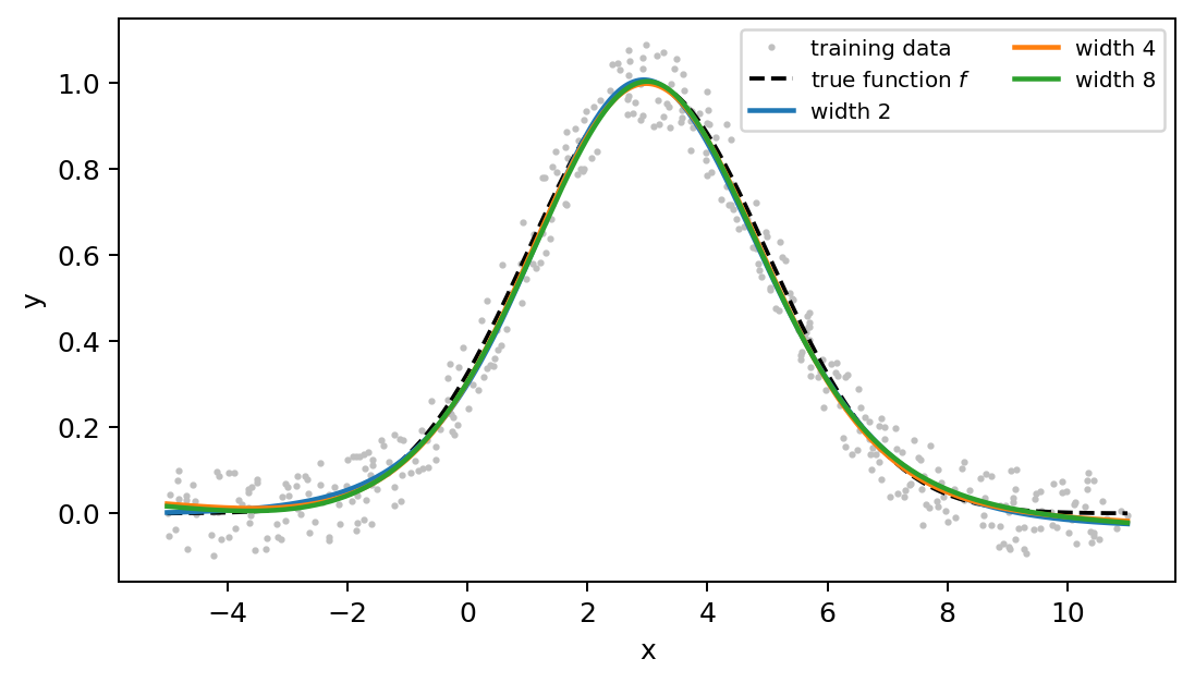
Fit this network for \(q=2,4,8\), with the same data, loss and optimizer as in Exercise 1. Report training and test MSE and plot the fits. How many neurons do you need before the fit is as good as the noise allows?
Solution
| widths | parameters | train MSE | test MSE |
|---|---|---|---|
| 2 | 7 | 0.00331 | 0.00388 |
| 4 | 13 | 0.00329 | 0.00376 |
| 8 | 25 | 0.00333 | 0.00382 |
Two neurons are enough: the training MSE of \(0.0033\) is the noise floor, so the fit is as good as it can be, and \(q=4\) and \(q=8\) do not improve it. Note that the \(q=2\) network has \(7\) parameters, fewer than the \(8\) of the three-layer stack of Exercise 1 that failed.
Exercise 4.
Why do two neurons suffice? Plot the two hidden units \(h_1(1)\) and \(h_1(2)\) of the fitted \(q=2\) network as functions of \(x\), together with the prediction \(\hat y\), and explain the mechanism.
Solution
Each hidden unit is a \(\tanh\) step. Both fitted units step up, but at different places: ours cross zero at \(x\approx 1.7\) and \(x\approx 4.1\), on the left and the right flank of the bump. The output weights are \(+1.09\) and \(-1.11\), so the output layer subtracts the second step from the first. A step up minus a later step up is a bump. This is what a single neuron cannot do: it has one step and nothing to subtract from it.
Exercise 5.
The universal approximation theorem says that one hidden layer of sufficient width can approximate any continuous function on a compact domain arbitrarily well. Exercise 1 shows a network that cannot approximate a bump at any depth. Are these two statements in conflict?
Solution
No. The theorem asks for width: the number of neurons \(q\) in the hidden layer must be allowed to grow. The stack of Exercise 1 keeps \(q=1\) and grows the depth instead, which the theorem says nothing about. The experiment is a concrete case of what the theorem’s condition is for.
7.1.4 Further questions about the bump
Exercise 6.
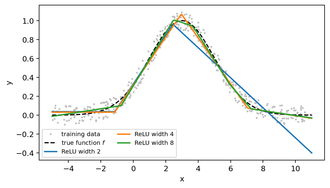
Replace \(\tanh\) by the ReLU everywhere and repeat Exercise 2. The fitted curve now looks different.
Solution
With ReLU activations the fitted curves are piecewise linear rather than smooth: each hidden unit introduces a kink. The output layer combines several hinges to make a piecewise-linear approximation to the bump. As before, the wider networks improve the fit; the difference is that their flanks now have straight segments rather than the smooth \(\tanh\) shape.
| width | parameters | train MSE | test MSE |
|---|---|---|---|
| 2 | 7 | 0.01436 | 0.01946 |
| 4 | 13 | 0.00408 | 0.00474 |
| 8 | 25 | 0.00341 | 0.00400 |
Two ReLU units make only a coarse, triangular approximation. Four and eight units have enough hinges to give a fit close to the noise floor.
Exercise 7.
Keep \(q=8\) but train on \(20\) points instead of \(400\). Compare the training MSE with the test MSE. What do you see, and which technique from the chapter would you use against it?
Solution
For the same random-number seed and training settings as above, we obtained
| training points | parameters | train MSE | test MSE |
|---|---|---|---|
| 20 | 25 | 0.00356 | 0.00370 |
There is no meaningful train–test gap in this run: the smooth bump is simple enough that twenty noisy observations still locate it well. This is a useful reminder that having more parameters than observations does not by itself prove overfitting. With a wider network, longer training, or an unlucky sample, a clear gap can appear. In that case use a validation set (or cross-validation) to choose regularization or early stopping; both limit fitting of the noise rather than the underlying bump.
7.2 Second-hand Toyota Corollas
The bump is a made-up function of one feature, chosen so that we can see what the network does. We now take real data with many features, where nobody knows the true \(f\), and where a competing method is available.
The file data/ToyotaCorolla.csv holds \(1436\) sales records of second-hand
Toyota Corollas. The target is Price, in euros.
Exercise 8.
Inspect the data before fitting a model. Which columns should you drop, and why? Do not rely only on the column names: inspect the values, data types, and number of distinct values first. Then identify which of the retained predictors are numerical and which are categorical.
Solution
Drop Id, which is essentially a row identifier; Cylinders, which is
constant (every car has four); and Mfg_Month and Mfg_Year, which together
reconstruct Age_08_04, apart from the dataset’s one-month convention. Also
drop Model: it contains 319 free-text labels for only 1436 rows, so one-hot
encoding it produces a sparse, high-cardinality feature that is not useful for
this exercise. Inspecting the data is essential here: a column that sounds
meaningful can be constant, an identifier can have almost one distinct value per
row, and duplicated date information is only apparent after comparing columns.
Exercise 9.
Decide which retained predictors are numerical and which are categorical. Why does this distinction matter for the preprocessing pipeline? Are any of the variables ordinal, and how would you represent them here?
Solution
Treat the following variables as numerical:
Age_08_04, KM, Weight, HP, Guarantee_Period, CC, Quarterly_Tax
They measure quantities for which a numerical difference has a meaning: for example, 10,000 additional kilometres or 100 additional kilograms. The other \(26\) retained variables are categorical, including the many binary equipment indicators. The pipeline scales numerical variables (for the neural network) and one-hot encodes categorical ones, so that arbitrary category labels are not mistaken for measurements or distances.
Doors and Gears have an ordering and can be called ordinal. In this small
dataset we still one-hot encode them: there is no reason to assume that the
effect of each extra door or gear is a constant linear increment in price. By
contrast, the numerical variables above may be discrete, such as age in months,
but they are still measured quantities with meaningful distances.
Split off \(20\%\) of the rows as a test set.
Prices have mean \(10731\) and standard deviation \(3627\). Predicting the mean price for every car gives a mean absolute error of \(2615\) on the test set. That is the number to beat; a model that does not beat it has learned nothing.
Exercise 10.
Fit a random forest to predict the price, and evaluate it.
- Do you need a random forest regressor or a random forest classifier?
- Do you have to scale the numerical features, as you do for ridge and lasso? Make sure you understand why, not just what the GPT answers.
- Build the forest. Use a pipeline to deal with the mix of categorical and numerical features. How is the depth of the trees determined, and how many features are tried per split?
- Plot the predicted against the observed prices on the test set, and plot the relative residuals.
- Make a bar plot of the most important features. How is the importance of a feature determined? Could you explain that to a manager?
Solution
With \(300\) trees and one-hot encoded categorical features we obtained a test MAE of \(741\) and a test RMSE of \(978\). Five-fold cross-validation gave MAEs of \(863, 778, 803, 735, 720\), so a mean of \(780\) and a spread of about \(\pm 70\) between folds.
An MAE of \(780\) on cars of average price \(10731\) is an error of about \(7\%\). Against the \(2615\) of the predict-the-mean baseline it is a factor of \(3.4\) better. Whether \(7\%\) is good enough is not a statistical question but a business one: it depends on the margin of the dealer.
Exercise 11.
Now predict the same prices with a neural network. Use the same split and the same preprocessing as for the forest, except that the numerical features must now be scaled. Fit an architecture without a hidden layer and see what you get. Then put in one hidden layer; take a width of \(10\), then of 30, then of \(100\). Report the test MAE and RMSE of each.
You may reuse your PyTorch code with \(p\) inputs instead of one, or use
MLPRegressor from sklearn, which is quicker to set up. Its default
activation is the ReLU.
Solution
With MLPRegressor, max_iter=4000 and everything else at its default:
| hidden layers | test MAE | test RMSE |
|---|---|---|
| predict mean | 2615 | 3655 |
| 1 | 1426 | 1910 |
| 1-1 | 824 | 1215 |
| 1-1-1 | 10613 | 11224 |
| 10 | 843 | 1238 |
| 100 | 839 | 1225 |
| 100-50 | 776 | 1160 |
| random forest | 741 | 978 |
Three things to notice. A single neuron already reaches \(1426\), far better than the baseline, whereas for the bump it was useless. The \(1\)-\(1\)-\(1\) network did not train at all: an MAE of \(10613\) is about what you get by predicting zero. And going from \(10\) to \(100\) neurons changes almost nothing, while the second layer in \(100\)-\(50\) helps a little.
Exercise 12.
Why does a single neuron do so much better here than it did on the bump, where we proved it could not work at all? Look at what the neuron receives as input.
Solution
In the bump problem there was one feature, so the neuron computed \(\hat y = a_2\tanh(a_1x+b_1)+b_2\), a monotone function of \(x\) itself, and the target was not monotone.
Here the neuron receives \(p=72\) inputs, the \(7\) numerical features and the one-hot columns of the \(26\) categorical ones, so it computes a monotone function of the linear combination \(w^{\top}x+b\). It can choose the direction \(w\): decreasing in age and kilometres, increasing in weight and horsepower. A car price is largely monotone in such an index, so this already explains a lot. What the single neuron still cannot do is represent interactions between features, i.e. the mileage mattering more for an old car than for a new one, since it has only one index available.
Exercise 13.
Compare the forest and the networks. Which method would you deliver to the dealer, and what would you tell them about how much to trust it? Bear in mind that with silly hyperparameters you can make either method look bad, so compare reasonable settings.
Solution
The forest wins on both numbers, at \(741\) against \(776\), and its RMSE is better by more: \(978\) against \(1160\), which says the network makes larger occasional mistakes. It also needs no scaling, no choice of width and depth, and trains in seconds, and it reports feature importances that the dealer can read.
The honest summary is that on a table of \(1436\) rows with \(40\) mostly categorical columns, a forest is the better tool, and the neural network is not obviously worth its extra tuning. Neural networks earn their keep where features are not given as a clean table, such as images, text or the token sequences of the language-model chapter.