4.7 Graphical Summaries

from pathlib import Path
import sys
sys.path.insert(0, str((Path.home() / "vakken" / "course-common" / "scripts").resolve()))
from render_tikz import render_tikz

render_tikz(r"""
\begin{tikzpicture}[node distance = 2.5cm]
\tikzset{
 >=stealth',
 pil/.style={
 ->,
 thick,
 shorten <=2pt,
 shorten >=2pt,}
}

\tikzstyle{block} = [rectangle, draw,text centered, rounded corners, minimum height=3em]

 \node [block, fill=red!50] (X_k) {$\{X_k\}$};
 \node [block, right=2.5cm of X_k,fill=red!50] (A_k) {$\{A_k\}$}
 edge[pil,bend left=45] node[below] {$X_k := A_k - A_{k-1}$} (X_k)
 edge[pil,<-, bend right=45] node[above] {$A_k := A_{k-1} + X_{k}$} (X_k);
 \node [block, right=2.5cm of A_k ] (A_t) {$\{A(t)\}$}
 edge[pil,bend left=45] node[below] {$A_k := \inf\{t: A(t)\geq k\}$} (A_k)
 edge[pil,<-, bend right=45] node[above] {$A(t) := \max\{k: A_k\leq t\}$} (A_k);
 \node [block, below=2cm of X_k ] (EX) {$\frac 1n \sum_{k=1}^n X_k \to \E X$}
 edge[pil, <-] (X_k);
 \node [block, below=2cm of A_t ] (lambda) {$\frac{A(t)}t \to \lambda$}
 edge[pil, <-] (A_t);
 \node [block, below=2cm of A_k ] {$\E X = \lambda^{-1}$}
 edge[pil, <-] (EX)
 edge[pil, <-] (lambda);

 \node[below=1cm of lambda] (dummy) {};

 \node [block, below=1cm of EX, fill=red!50] (S_k) {$\{S_k\}$};
 \node [block, right=2.5cm of S_k ] (U_k) {$\{U_k\}$}
 edge[pil,<->] (S_k);
 \node [block, right=2.5cm of U_k ] (U_t) {$\{U(t)\}$}
 edge[pil,<->] (U_k);
 \node [block, below=1cm of S_k ] (ES) {$\frac 1n \sum_{k=1}^n S_k \to \E S$}
 edge[pil, <-] (S_k);
 \node [block, below=1cm of U_t ] (mu) {$\frac{U(t)}t \to \mu$}
 edge[pil, <-] (U_t);
 \node [block, below=1cm of U_k ] {$\E S = \mu^{-1}$}
 edge[pil, <-] (ES)
 edge[pil, <-] (mu);

 \node [block, right=of dummy] {Stability:\newline $\lambda < \mu$}
edge[pil,bend right=25, <-] (lambda.east)
edge[pil,bend left=25, <-] (mu.east);

 \node[block, below=1cm of ES, fill=red!50 ] (W_k) {$\J_{k}=\max\{\J_{k-1} - X_k,0\} +S_k$};
 \draw[->] (S_k.west) [out=180, in=110] to (W_k.north west);
 \draw[->] (X_k.west) [out=230, in=110] to (W_k.north west);
 \node[block, right=1cm of W_k, fill=red!50 ] (D_k) {$D_{k}=A_k + \J_{k}$}
 edge[pil,bend right=25, <-] (A_k)
 edge[pil,<-] (W_k);
 \node[block, right=1cm of D_k ] (D_t) {$D(t)=\max\{k: D_k\leq t\}$}
 edge[pil, <-] (D_k);

 \node[block, below=1cm of W_k, fill=blue!40] (W) {$\frac1n\sum_{k=1}^n \W_k \to \E\W$}
 edge[pil, <-] (W_k);
 \node[block, below=1cm of D_t] (Q_t) {$L(t) := A(t) - D(t)$}
 edge[pil, <-] (D_t);
 \draw[->] (A_t.east) [out=20, in = 40] to (Q_t);

 \node[block, right=1cm of D_t] (delta) {$\frac{D(t)}t \to \delta$}
 edge[pil, <-] (D_t);
 \node[block, below=1cm of D_k, fill=blue!40] (L) {$\frac 1 t \int_0^t L(s)\,\d s \to \E\L$}
 edge[pil, <-] (Q_t);

 \node[block, right=1cm of Q_t] (hoi) {$\delta \leq \lambda$}
 edge[pil, <-] (delta)
 edge[pil, bend right=10, <-] (lambda)
 edge[pil, bend left = 30, <-] node[below] {$L(t)>0$} (Q_t);

 \node[block, below=1cm of W, fill=blue!40] (PW) {$\frac 1n \sum_{k=1}^n \1{\W_k \leq w} \to \P{\W\leq w}$}
 edge[pil, <-] (W);

 \node[block, below=1cm of Q_t, fill=blue!40] (PL) {$\frac 1t \int_{0}^t \1{\L(s) \leq l} \to \P{\L\leq l}$}
 edge[pil, <-] (Q_t);

\end{tikzpicture}
""", "../figures/construction_gg1.png")
construction_gg1.png
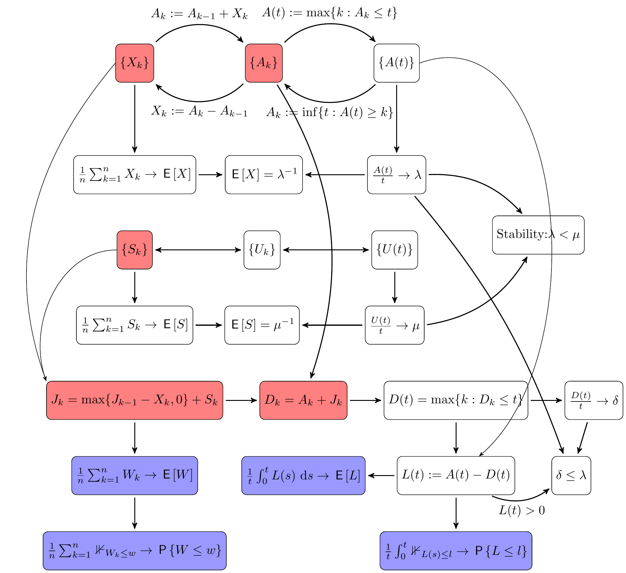
Figure 4.1: An overview of the relations between the different types of times (inter-arrivals, arrivals, departures and so on) we use to construct a queueing process in continuous time.
from pathlib import Path
import sys
sys.path.insert(0, str((Path.home() / "vakken" / "course-common" / "scripts").resolve()))
from render_tikz import render_tikz

render_tikz(r"""
\begin{tikzpicture}[node distance = 2.5cm]
\tikzset{
 >=stealth',
 pil/.style={
 ->,
 thick,
 shorten <=2pt,
 shorten >=2pt,}
}
\tikzstyle{block} = [rectangle, draw,text centered, rounded corners, minimum height=3em]

 \node [block, text width=5.5cm, align=center] (level) {Counting};
\node[block, below=1cm of level] (An) {$|A(n,t)-D(n,t)|\leq 1$}
edge[pil,<-] (level);

\node[block, left=1.5cm of An] (A) {$A(t)-D(t)=\L(t)$}
edge[pil,<-] (level);

\node[block, below=1cm of A] (At) {$\frac{A(t)}t \approx \frac{D(t)}t$ if $\frac{\L(t)}t \to 0$}
edge[pil,<-] (A);

\node[block, below=1.5cm of At] (lambda) {$\lambda=\delta$}
edge[pil,<-] node[fill=white] {$t\to\infty$} (At);

\node[block, below=1cm of An] (AnDn) {$\frac{A(n,t)}t\approx\frac{D(n,t)}t$}
edge[pil,<-] (An);

\node[block, below=1.5cm of AnDn] (AnDn2) {$\frac{A(n,t)}{Y(n,t)}\frac{Y(n,t)}t\approx\frac{D(n,t)}{Y(n+1)}\frac{Y(n+1)}t$}
edge[pil,<-] (AnDn);

\node[block, below=1.5cm of AnDn2, text width=4cm] (lp) {Level Crossing: \\
$\lambda(n)p(n) = \mu(n+1)p(n+1)$}
edge[pil,<-] node[fill=white] {$t\to\infty$} (AnDn2);

\node[block, below=1cm of lp, text width=3cm] (poisson) {Poisson: \\
$\lambda=\lambda(n)$, \\
$\mu=\mu(n)$}
edge[pil,<-] (lp);

\node[block, below=1cm of poisson, text width=4cm] (mm1) {$M/M/1$, $M/M/c$, $M/M/c/k$, \ldots} edge[pil,<-] (poisson);
;

\node[block, right=0.6cm of lp, text width=5cm, align=center] (batch) {$\lambda\sum_{m=0}^nG(n-m)p(m) = \mu(n+1)p(n+1)$}
edge[pil,<-] (lp);

\node[block, right=2.3cm of mm1] (batch2) {$M^B/M/1$}
edge[pil,<-] (poisson)
edge[pil,<-] (batch);
\node[block, below=1cm of mm1, text width=4.5cm] (perf) {Performance
 measures:
$\E \L= \sum_{n=0}^\infty n p(n)$, $\P{\L\geq m}$, \ldots}
edge[pil,<-] (mm1)
edge[pil,<-] (batch2);

\node[block, below=1.5cm of lambda] (pasta1) {$\frac{A(t)}t\frac{A(n,t)}{A(t)} = \frac{A(n,t)}{Y(n,t)}\frac{Y(n,t)}t$}
edge[pil,<-] (AnDn2)
edge[pil,<-,bend left=20] (At.south west)
;

\node[block, below=1.5cm of pasta1] (pasta2) {$\lambda \pi(n) = \lambda(n)p(n)$}
edge[pil,<-] node[fill=white] {$t\to\infty$} (pasta1);

\node[block, below=1.5cm of pasta2, text width=3cm] (pasta3) {PASTA: $\pi(n) = p(n)$}
edge[pil,<-] (poisson)
edge[pil,<-] (pasta2)
edge[pil,->] (perf);

\end{tikzpicture}
""", "../figures/level_crossing_summary.png")
level_crossing_summary.png
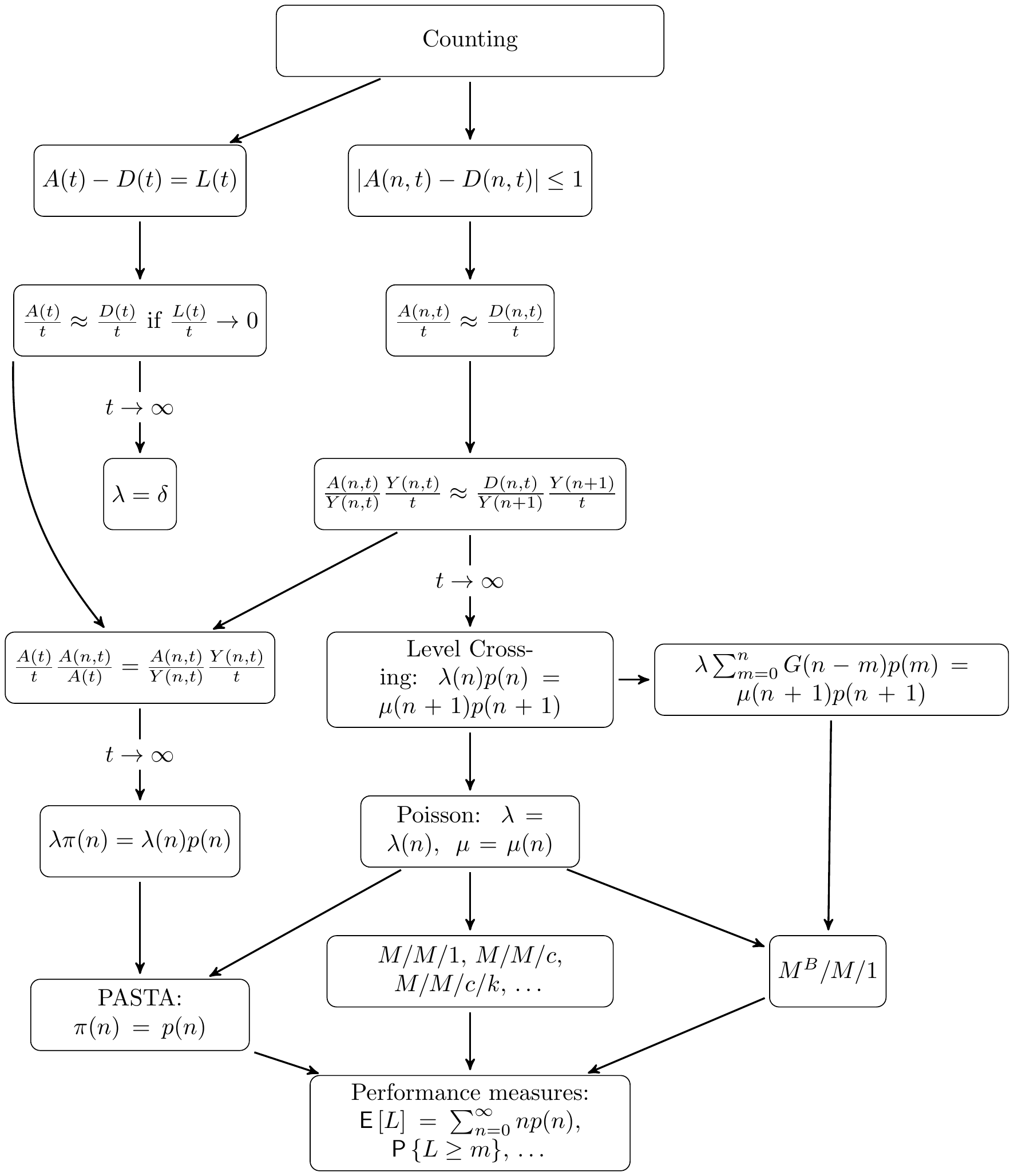
Figure 4.2: This figure presents an overview of the results that derive from level-crossing arguments.