
7.5 Mean Value Analysis of Closed Queueing Networks (UNDER CONSTRUCTION)
7.5 Mean Value Analysis of Closed Queueing Networks (UNDER CONSTRUCTION)
We now consider a closed network with \(n\) circulating jobs. There are \(m\) single-server, first-come-first-served stations. The service time \(S_i\) at station \(i\) is exponentially distributed, with mean \(\E{S_i}.\) Jobs follow fixed or Markov routing. We take station 1 as the reference station and let \(V_i\) be the mean number of visits to station \(i\) per visit to station 1, so \(V_1=1.\)
Let \(\L_i(n)\) be the stationary number of jobs at station \(i,\) including any job in service, and \(\J_i(n)\) the time a job spends there per visit. The throughput at station \(i\) is \(\TH_i(n).\) We compute these measures for populations \(n=1,\ldots,N.\)
The arrival theorem says that when a job arrives at station \(i\) in a closed network with \(n\) jobs, the other jobs it sees have the same stationary distribution as the jobs in the network with only \(n-1\) jobs. In particular, the mean number it sees at station \(i\) is \(\E{\L_i(n-1)}.\) This result holds for the product-form closed network considered here; it is not an assumption that arrivals form a Poisson process. Recall from Section 7.3 that the inter-departure times of a stationary \(M/M/1\) queue with Poisson arrivals are \(\Exp{\lambda}.\) The arrival theorem instead describes the queue lengths seen by a job moving through a closed network.
If the arriving job finds \(q\) jobs at station \(i,\) it must wait for those \(q\) services and then receive its own service. The exponential distribution is memoryless, so the remaining service time of a job already in service also has mean \(\E{S_i}.\) Hence the mean time spent at station \(i\) is
\begin{equation*} \E{\J_i(n)} = \bigl(1+\E{\L_i(n-1)}\bigr)\cdot\E{S_i}, \qquad n\geq 1. \tag{7.5.1} \end{equation*}The mean cycle time for a visit to station 1 and return is \(\E{\J(n)}=\sum_{i=1}^m V_i\cdot\E{\J_i(n)}.\) Little’s law for the whole closed network gives \(n=\TH_1(n)\cdot\E{\J(n)}.\) The station throughputs follow from the visit ratios, and Little’s law at each station then gives
\begin{alignat*}{3} \TH_1(n) &= \frac{n}{\E{\J(n)}},\quad & \TH_i(n) &= V_i\cdot\TH_1(n),\quad & \E{\L_i(n)} &= \TH_i(n)\cdot\E{\J_i(n)}. \tag{7.5.2} \end{alignat*}We start with \(\E{\L_i(0)}=0.\) Equation (7.5.1) supplies \(\E{\J_i(1)},\) which gives \(\TH_i(1)\) and \(\E{\L_i(1)}.\) Repeating this step for \(n=2,3,\ldots\) yields the performance measures for any desired population. The equations are exact under the assumptions above.
For example, take two stations. Let \((\E{S_1},\E{S_2})=(2,1)\) and \((V_1,V_2)=(1,1).\) The first three steps give
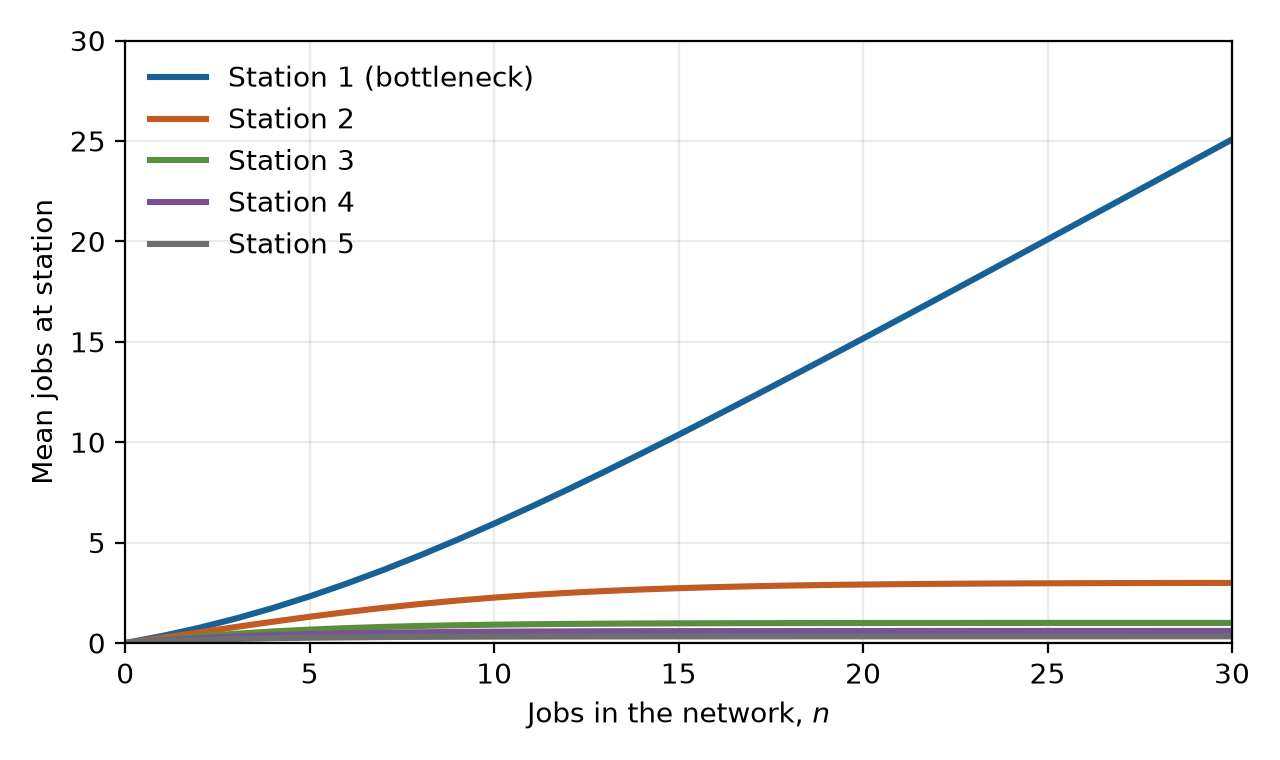
\begin{center} \begin{tabular}{c|ccc} \(n\) & \(\TH_1(n)\) & \(\E{\L_1(n)}\) & \(\E{\L_2(n)}\) \\ \hline 0 & 0 & 0 & 0 \\ 1 & \(1/3\) & \(2/3\) & \(1/3\) \\ 2 & \(3/7\) & \(10/7\) & \(4/7\) \\ 3 & \(7/15\) & \(34/15\) & \(11/15\) \end{tabular} \end{center}At each step, \(\E{\L_1(n)}+\E{\L_2(n)}=n,\) as it must: all \(n\) jobs are at one of the two stations. With five stations the buildup at a bottleneck is clearer. Take mean service times \(2,3/2,1,3/4,1/2\) at stations 1 through 5, respectively. Each station is visited once per cycle. Fig. 7.1 shows that the mean populations at the four faster stations level off, while almost every additional job joins station \(1.\)
In a CONWIP line each job on the shop floor holds a card. When a job leaves, its card permits another job to enter. If new work is always waiting and the card is reused immediately, \(n\) cards keep exactly \(n\) jobs in the line. MVA then gives the throughput \(\TH_1(n)\) and the mean cycle time \(\E{\J(n)}=n/\TH_1(n).\) Computing these measures for several card counts shows how much extra throughput we gain by allowing more work in process, and how much longer jobs spend in the line.
We can compute populations in order. A cache is useful when we ask for several populations, perhaps in a different order. For example, after computing the result for \(n=2,\) a request for \(n=3\) can reuse it; another request for \(n=2\) returns immediately.
The function below uses the cache and membership test from Alg. 1.2.21, and the default-zero map from Alg. 1.2.13. It returns a function \(\pr{mva}\) that retains \(\var{cache}.\) Each entry \(\var{cache}(n)\) stores the reference-station throughput and a map of mean station populations.
\begin{algorithm}
\caption{Compute mean value analysis results and cache them by population.}
\begin{algorithmic}[1]
\State \textbf{Input:} mean service times \(\E{S_i}>0,\) visit ratios \(V_i\geq0,\) \(1\leq i\leq m,\) with \(V_1=1\).
\State \textbf{Output:} a function \(\pr{mva}(n)\) returning \(\TH_1(n)\) and \(\E{\L_i(n)},\) \(1\leq i\leq m\).
\Function{MVA}{\((\E{S_i})_{i=1}^m,\, V\)}
    \State \((\var{cache},\, \pr{InCache?})\gets\pr{Cache}()\)
    \State \(\var{cache}(0)\gets\bigl(0,\, \pr{Map}()\bigr)\) \Comment{At population zero, every station is empty.}
    \Function{mva}{\(n\)}
        \If{\(\pr{InCache?}(n)\)}
            \Return \(\var{cache}(n)\)
        \EndIf
        \State \((\TH_{\mathrm{old}},\, L_{\mathrm{old}})\gets\pr{mva}(n-1)\)
        \State \(J\gets\pr{Map}(),\) \(L\gets\pr{Map}(),\) \(T\gets0\)
        \For{\(1\leq i\leq m\)}
            \State \(J(i)\gets\bigl(1+L_{\mathrm{old}}(i)\bigr)\cdot\E{S_i}\) \Comment{Arrival theorem.}
            \State \(T\xleftarrow{+}V_i\cdot J(i)\)
        \EndFor
        \State \(\TH_1\gets n/T\) \Comment{Little's law for the network.}
        \For{\(1\leq i\leq m\)}
            \State \(L(i)\gets V_i\cdot\TH_1\cdot J(i)\) \Comment{Little's law at station \(i.\)}
        \EndFor
        \State \(\var{cache}(n)\gets(\TH_1,\, L)\)
        \Return \(\var{cache}(n)\)
    \EndFunction
    \Return \(\pr{mva}\)
\EndFunction
\end{algorithmic}

\end{algorithm}
For the two-station example, let \(\pr{mva}\gets\pr{MVA}((2,1),(1,1)).\) The call \(\pr{mva}(2)\) fills \(\var{cache}(0),\var{cache}(1),\var{cache}(2).\) A subsequent call \(\pr{mva}(3)\) computes only the new entry \(\var{cache}(3).\) Repeating \(\pr{mva}(2)\) simply retrieves \(\var{cache}(2).\)