7 Neural Networks

The simplest neural network consists of a single neuron taking a single feature \(x\) as input and producing one prediction \(\hat y\). Fig. 7.1 shows the two steps. It does this by first computing the logit (5.1.3)

\begin{align*} z = ax+b, \end{align*}

with the weight \(a\) and bias \(b\). Then it applies an activation function to obtain the output \(\hat y \in \Yset\). Throughout this chapter we use the sigmoid as an example,

\begin{align*} \hat y = \sigma(z), \qquad \sigma(z) = \rb{1+e^{-z}}^{-1}. \end{align*}

The role of \(\sigma\) is to transform the unbounded logit \(z\in\R\) into a number between \(0\) and \(1\), so that \(\hat y\) can be interpreted as a probability. Thus, once \(a\) and \(b\) are known, prediction is just the calculation above. Note that the mechanism we describe below can be easily changed to other activation functions.

⊕
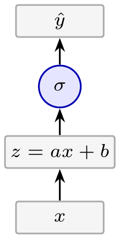
Figure 7.1: A single neuron computes a logit \(z\) from the input \(x\) and passes it through the activation function \(\sigma\) to obtain the response \(\hat y\).

For training we use the observations \((x,y)\) in the training set \(\Tset\). The goal is to solve the problem:

\begin{align*} \theta^{*} &\in \argmin_{\theta} \hat R_{\Tset}(a,b), & \theta &= (a,b), \tag{7.1.1} \end{align*}

where the training risk is the average over the training samples,

\begin{align*} \hat R_{\Tset}(a,b) &= \frac{1}{|\Tset|}\sum_{(x,y)\in\Tset}\lscr(y, f_{\theta}(x)), & f_{\theta}(x)&=\hat y=\sigma(ax+b), \end{align*}

and \(\lscr(y, \hat y)\) is the loss of the prediction \(\hat y\) on the single training sample \((x,y)\). Below we use squared-error loss

\begin{align*} \lscr(y,\hat y) = \frac{1}{2}\rb{y - \hat y}^{2}= \frac{1}{2}\rb{y - \sigma(ax+b)}^{2}. \end{align*}

For hard labels \(y\in\set{0,1}\) and soft targets \(y\in[0,1]\), binary cross-entropy (5.1.5) is a natural choice for \(\lscr\).

In practice, we use the gradient descent tools of Section 5.1 to search for a parameter vector with low training risk. Because the objective may be nonconvex, gradient descent may reach a local minimum rather than a global one. The resulting parameter vector is then used for prediction: for a new predictor \(x\), the neuron returns \(\sigma(a^* x + b^*)\) as the prediction.

Regularization is important even for this single neuron network; however, these ideas apply more generally.

Early stopping uses a validation set to decide when to stop training. Split the available labeled data into a training set \(\Tset\) and a validation set \(\Vset\). The parameters are updated by gradient descent on \(\hat R_{\Tset}\) as before, but now, at each iteration \(k\), we store the validation risk

\begin{align*} \hat R_{\Vset}(\theta^{(k)}) = \frac{1}{|\Vset|}\sum_{(x,y)\in\Vset}\lscr(y, f_{\theta^{(k)}}(x)) \end{align*}

together with the parameters \(\theta^{(k)}=(a^{(k)},b^{(k)})\). When the validation risk has failed to improve for a number of successive iterations, we stop iterating and use

\begin{align*} k^* \in \argmin_k \hat R_{\Vset}(\theta^{(k)}) \end{align*}

to select \(\theta^{(k^*)}\) as the fitted parameter vector for prediction instead of the last parameter values obtained from training. This matters because the training risk can keep decreasing, while the validation risk can increase once the model begins to fit accidental details of \(\Tset\).

Weight decay copies the idea from ridge regression by including a penalty in the objective:

\begin{align*} \min_{a,b}\hat R_{\Tset,\lambda}(a,b), \qquad \hat R_{\Tset,\lambda}(a,b) = \hat R_{\Tset}(a,b) + \frac{\lambda}{2}a^2, \end{align*}

where \(\lambda\geq 0\) is a tuning parameter.²²In larger networks, the weight \(a\) is a matrix. Then we penalize the sum of the squared entries of the weight matrix, \(\norm{A}^2\), instead of just \(a^2\).

The bias \(b\) is often left out of the penalty. The reason is that \(a\) controls the steepness of \(\sigma(ax+b)\), while \(b\) controls where the steep part of the curve lies.³³\(ax+b=0\) at \(x=-b/a\). Penalizing \(a\) discourages overly sharp changes in the fitted probabilities. Penalizing \(b\) would also discourage moving the steep part of the curve to where the data place it, which is usually not the intended effect.

The extra term in the objective contributes \(\lambda a\) to the derivative with respect to \(a\), so the update in gradient descent contains a small shrinkage toward zero. As \(\frac{\partial}{\partial a}\hat R_{\Tset,\lambda}(a,b)=\frac{\partial}{\partial a}\hat R_{\Tset}(a,b)+\lambda a\), the update for \(a\) is

\begin{align*} a^{(k+1)} &= a^{(k)} -\eta\left( \frac{\partial}{\partial a}\hat R_{\Tset}(a^{(k)},b^{(k)}) +\lambda a^{(k)} \right)\\ &= (1-\eta\lambda)a^{(k)} -\eta\frac{\partial}{\partial a}\hat R_{\Tset}(a^{(k)},b^{(k)}). \end{align*}

The first term is a shrunken version of the old value \(a^{(k)}\), before the usual gradient of the training risk is added. For the decay term alone to reduce the magnitude of the old weight, we need \(|1-\eta\lambda|<1\). This condition by itself does not ensure convergence of the full update; gradient-descent convergence depends on the objective and step size, among other assumptions.⁴⁴Wikipedia: Gradient descent.

A single neuron only gives shifted and stretched copies of one fixed nonlinearity, \(\sigma(ax+b)\). Neural networks become more flexible by combining many such transformations: some are placed in a sequence of layers, making the network deeper, and some are placed side by side, making a layer wider. Networks built from multiple layers, each of several neurons wide, are called multilayer perceptrons.

Making networks deeper and wider can improve prediction quality. Different hidden neurons can learn different useful patterns in the input, and later layers can combine patterns learned by earlier layers. However, if the network is made too large for the amount of data, the same flexibility can overfit by picking up accidental noise instead of structure.

We first study depth in the simplest case: a scalar stack with one neuron per layer. Then we make the network wider, and introduce more indices to cope with the extra complexity.

The simplest stack passes information from single neurons from one layer to the next, see Fig. 7.2. For instance, starting from the input \(x\), define

\begin{equation*} \begin{aligned} z_1 &= a_1x+b_1, & h_1 &= \phi_1(z_1),\\ z_2 &= a_2h_1+b_2, & h_2 &= \phi_2(z_2),\\ z_3 &= a_3h_2+b_3, & h_{3} &= \sigma(z_3), \\ \hat y &= h_{3}. \end{aligned} \tag{7.2.1} \end{equation*}

Each \(a_i\) and \(b_i\), for \(i=1,2,3\), is a trainable parameter; \(\phi_1\) and \(\phi_2\) are activation functions, in the same role as \(\sigma\).⁵⁵We discuss examples below. The intermediate values \(h_1\) and \(h_2\) are called hidden as the network only uses them internally. The \(z_i\) are the pre-activations; the last one, \(z_3\), is the logit. Since the signal flows only forward, from \(x\) through \(h_1\), \(h_2\) and \(h_{3}\) to \(\hat y\), without cycles or feedback, such a network is called feedforward. The value \(h_3\) of the last layer is not hidden, but we add it to simplify the derivations below considerably.

⊕
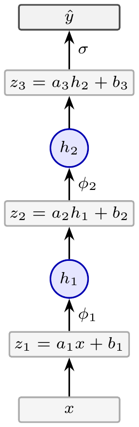
Figure 7.2: A scalar multilayer network.

This stack is richer than a single neuron because each layer transforms the signal once more, so a later layer works with features produced by the earlier layers rather than with the raw input.

Prediction is implemented as a forward pass. Given parameters \((a_i, b_i)\) for each neuron, compute for the predictor \(x\) the preactivations \(z_1, h_1, z_2, h_2, z_3\) in order of (7.2.1) and return \(\hat y=\sigma(z_3)\).

Training minimizes the training risk by (mini-batch) gradient descent, now over all six parameters \(\theta=(a_1,b_1,a_2,b_2,a_3,b_3)\). The new difficulty is computing the gradient. Backpropagation⁶⁶Michael A. Nielsen, Neural Networks and Deep Learning is the systematic way to handle this: it is the chain rule, applied from the output back to the input.

First, apply a forward pass to one observation \((x,y)\) to compute the prediction \(f_\theta(x)=\hat y\), the loss \(\lscr(y, f_\theta(x))\), all pre-activations \(z_i\) and all hidden values \(h_i\). The computations below use these values.

Backpropagation starts at the output, that is, at the top of Fig. 7.2. Let

\begin{align*} \delta_{3} = \frac{\partial \lscr(y, h_{3})}{\partial h_3}. \tag{7.2.2} \end{align*}

If we use square loss, \(\delta_{3} = (\hat y -y)\). As the parameters \(a_3\) and \(b_3\) enter the loss only through \(z_3=a_3h_2+b_3\), by the chain rule,

\begin{align*} \frac{\partial \lscr}{\partial a_3} &= \frac{\partial \lscr}{\partial h_{3}} \frac{\partial h_3}{\partial z_3} \frac{\partial z_3}{\partial a_3} = \delta_3 \sigma'(z_{3})h_2, & \frac{\partial \lscr}{\partial b_3} &= \frac{\partial \lscr}{\partial h_3} \frac{\partial h_3}{\partial z_3} \frac{\partial z_3}{\partial b_3} = \delta_3 \sigma'(z_{3}). \end{align*}

Note that from the forward pass we have the numerical values of \(\delta_3\), \(\sigma'(z_3)\), and \(h_2\) at the given sample \((x,y)\). Thus, the RHSs are just numbers that we⁷⁷That is, the computer. can compute.

Now step one layer back. From (7.2.1) and the chain rule⁸⁸Another way is to consider \(\frac{\partial \lscr}{\partial z_2} = \frac{\partial \lscr}{\partial z_3} \frac{\partial z_3}{\partial z_2}\). In view of the residual connections we discuss below, this decomposition does not work well.

\begin{align*} \delta_2 &=\frac{\partial \lscr}{\partial h_2} = \frac{\partial \lscr}{\partial h_3} \frac{\partial h_3}{\partial h_2} = \delta_{3} \sigma'(z_3) a_{3} \tag{7.2.3} \end{align*}

Since \(z_2=a_2h_1+b_2\), again by the chain rule,

\begin{align*} \frac{\partial \lscr}{\partial a_2} &= \frac{\partial \lscr}{\partial h_2} \frac{\partial h_2}{\partial z_2} \frac{\partial z_2}{\partial a_2} = \delta_2 \phi_2'(z_2) h_1, & \frac{\partial \lscr}{\partial b_2} &= \frac{\partial \lscr}{\partial h_2} \frac{\partial h_2}{\partial z_2} \frac{\partial z_2}{\partial b_2} = \delta_2 \phi_2'(z_2). \end{align*}

One more step of the same kind yields

\begin{align*} \delta_1 &= \frac{\partial \lscr}{\partial h_2} \frac{\partial h_2}{\partial h_1} = \delta_2 \phi_2'(z_2) a_2, \tag{7.2.4} \end{align*}

and by the same token

\begin{align*} \frac{\partial \lscr}{\partial a_1} &= \frac{\partial \lscr}{\partial h_1} \frac{\partial h_1}{\partial z_1} \frac{\partial z_1}{\partial a_1} = \delta_1 \phi_1'(z_1) x, & \frac{\partial \lscr}{\partial b_1} &= \frac{\partial \lscr}{\partial h_1} \frac{\partial h_1}{\partial z_1} \frac{\partial z_1}{\partial b_1} = \delta_1 \phi_1'(z_1). \end{align*}

For the plain network above, note the pattern: One forward pass computes the \(z_i\) and hidden values \(h_i\), one backward pass computes each \(\delta_i\), and from these \(\partial_{a_i} \lscr\) and \(\partial_{b_i} \lscr\). Together they deliver the complete gradient \(\nabla_\theta\lscr(y, f_\theta(x))\) for the given sample \((x,y)\).

The parameter update is then the same as before, except that rather than updating from just one sample, we use a mini-batch \(\Bset\) to estimate the gradient with (5.1.6) and update the parameters through:

\begin{align*} \theta^{(k+1)} = \theta^{(k)} - \eta\, \nabla\hat R_{\Bset}(\theta^{(k)}) = \theta^{(k)} - \eta\, \frac{1}{|\Bset|} \sum_{(x,y) \in \Bset} \left.\nabla_{\theta} \lscr(y, f_{\theta}(x))\right|_{\theta=\theta^{(k)}}. \tag{7.2.5} \end{align*}

For instance, for a mini-batch containing a single sample,

\begin{align*} a^{(k+1)}_{1} &= a^{(k)}_{1} - \eta \frac{\partial \lscr}{\partial a_1} = a^{(k)}_{1} - \eta \delta_1\phi_1'(z_1)x, & b^{(k+1)}_{1} &= b^{(k)}_{1} - \eta \frac{\partial \lscr}{\partial b_1} = b^{(k)}_{1} - \eta \delta_1\phi_1'(z_1). \end{align*}

The other parameters follow in the same way.

Because the training risk of a neural network is not necessarily convex, two runs started from different initial parameter values may end at different local minima. A simple practical response is to train the same architecture from several random initializations and keep the run with the lowest validation risk.

Generalizing to networks with \(L\) layers, including the output layer, is straightforward. Thus there are \(L-1\) hidden layers.

Widening a layer places several neurons side by side in one layer, see Fig. 7.3. A neuron in a wide layer now receives several inputs, one from every neuron in the previous layer, so its weights carry three indices: \(A_i(j,k)\) is the weight that neuron \(j\) of layer \(i\) applies to its \(k\)-th input. Then hidden layer \(i\) computes the components of its pre-activation and hidden vector as

\begin{align*} z_i(j)&=\sum_{k=1}^{q_{i-1}} A_i(j,k)h_{i-1}(k) + b_i(j), & h_i(j) &= \phi_i(z_i(j)). \tag{7.2.6} \end{align*}

Collecting the weights of layer \(i\) in the matrix \(A_i\in\R^{q_i\times q_{i-1}}\), whose \((j,k)\) entry is \(A_i(j,k)\), the hidden vector \(h_{i-1}\in \R^{q_{i-1}}\), and the biases in the vector \(b_i\in\R^{q_i}\), this becomes

\begin{align*} z_i &= A_i h_{i-1} + b_i, & h_i &=\phi_i(z_i), & i&=1,\ldots,L-1, \tag{7.2.7} \end{align*}

where \(\phi_i\) is applied element-wise. The output is layer \(L\). It consists of one neuron, so \(q_L=1\), and it reads the last hidden layer,

\begin{align*} z_L &= A_Lh_{L-1} + b_L, & \hat y &= \sigma(z_L) \tag{7.2.8} \end{align*}

with \(A_L\in\R^{1\times q_{L-1}}\) and \(b_L\in\R\). Thus the output layer has the same affine form as a hidden layer, with the output activation \(\sigma\).

⊕
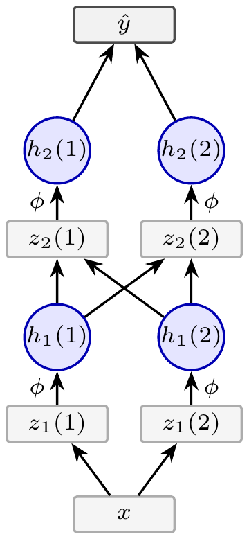
Figure 7.3: A small multilayer perceptron.

Each layer has its own parameters \(A_i(j,k), b_i(j)\); thus

\begin{align*} \theta=(A_1,b_1,\ldots,A_L,b_L). \end{align*}

Note how quickly \(\theta\) grows: layer \(l\) alone has \(q_l(q_{l-1}+1)\) parameters.

Including multiple features is now straightforward. When the input is a feature vector \(x\in\R^p\), just set \(h_0=x\) and \(q_0=p\), and all of (7.2.7) applies right away. Thus, moving from one to \(p\) features changes only the bookkeeping for the first layer; later layers are unaffected as they read only from the previous hidden layer.

Backpropagation carries over nearly unchanged. Again, there is one \(\delta\) per neuron, so \(\delta_i\in\R^{q_i}\) is a column vector, as are \(h_i\), \(z_i\) and \(b_i\). The output layer \(L\) has one neuron, so

\begin{align*} \delta_L = \frac{\partial \lscr}{\partial h_L}. \end{align*}

The other backward recursions follow from the chain rule:

\begin{align*} \delta_i(j) &= \frac{\partial \lscr}{\partial h_i(j)} = \sum_{k}\frac{\partial \lscr}{\partial h_{i+1}(k)} \frac{\partial h_{i+1}(k)}{\partial h_i(j)} \\ &= \sum_{k} \delta_{i+1}(k) A_{i+1}(k,j) \phi_{i+1}'(z_{i+1}(k)), \end{align*}

where we use (7.2.6) for the second partial derivative and \(h_{i+1}(k) = \phi_{i+1}(z_{i+1}(k))\) for the third. Now note that the summation over \(k\) is the \(j\)-th component of \(A_{i+1}^{\top}\rb{\delta_{i+1} \odot \phi_{i+1}'(z_{i+1})}\). With the Hadamard product⁹⁹The Hadamard product, written as \(C = A \odot B\), of two matrices \(A\) and \(B\) with the same dimensions is the element-wise multiplication: \(C_{ij} = A_{ij} B_{ij}\). we can then write

\begin{align*} \delta_i = A_{i+1}^{\top}\rb{\delta_{i+1} \odot \phi_{i+1}'(z_{i+1})}, \qquad i = L-1,\ldots,1. \end{align*}

Finally, the gradients of layer \(i=1,\ldots,L\) become

\begin{align*} \frac{\partial \lscr}{\partial A_i} &= \rb{\delta_i \odot \phi_i'(z_i)}\, h_{i-1}^{\top}, & \frac{\partial \lscr}{\partial b_i} &= \delta_i \odot \phi_i'(z_i), \end{align*}

because

\begin{align*} \frac{\partial \lscr}{\partial A_i(j,k)} &= \frac{\partial \lscr}{\partial h_i(j)} \frac{\partial h_i(j)}{\partial z_i(j)} \frac{\partial z_i(j)}{\partial A_i(j,k)} = \delta_i(j)\phi_i'(z_i(j))h_{i-1}(k). \end{align*}

These are the gradients for one observation. For a mini-batch, average each of these per-observation gradients over the batch before updating the parameters, just as in (7.2.5).

As an aside, in software these formulas need not be derived by hand: automatic differentiation records every elementary operation of the forward pass and applies the chain rule mechanically in reverse, which reproduces exactly the backpropagation computation above, for a network of any shape. This is what allows practitioners to change an architecture without redoing any calculus. Also, in real large networks, plain gradient descent is often replaced by specialized optimizers such as momentum methods, Adam, or AdamW.¹⁰¹⁰Wikipedia: Stochastic gradient descent, Adam.

Multi-neuron networks can use other regularization techniques besides early stopping and weight decay.

Dropout is a technique that aims to prevent the network from relying too much on just a few neurons in a layer. The risk with \(q\) parallel neurons is that during training they can start to cooperate too closely so that just a few neurons in that layer become dominant, which in turn may lead to tuning that layer to accidental details of the training set. Dropout counters this by switching off neurons selected at random for each training sample, see Fig. 7.4. Like this, the network cannot rely on just a few neurons; in that sense, it should make networks more robust.

⊕
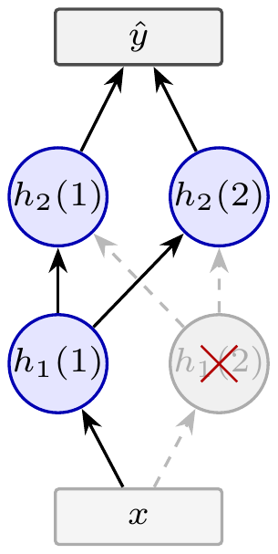
Figure 7.4: Dropout switches off hidden units during training.

Dropout is generally applied to each hidden layer separately; we discuss the details for one layer. Given the vector \(h_i\) of hidden layer \(i\), let \(\rho\in[0,1)\) be the dropout probability. For each sample in a mini-batch, independently draw a mask \(M_i=(M_i(1),\ldots,M_i(q_i))\) where

\begin{align*} M_i(j)\sim \Bern{1-\rho}, \quad j=1,\ldots,q_i \end{align*}

are independent mask variables.¹¹¹¹In deeper networks, use a separate mask for each dropout layer. Then, replace \(h_i\) by its randomly thinned version

\begin{align*} \tilde h_i = \frac{M_i\odot h_i}{1-\rho}, \end{align*}

and use \(\tilde h_i\) instead of \(h_i\) in (7.2.7). Thus, each sample is processed by a differently thinned network. Since the model cannot rely on the same hidden units always being present, no single neuron can play too dominant a role.

The division by \(1-\rho\) is called inverted dropout. It keeps \(\E{\tilde h_i(j)}=h_i(j)\), so that in expectation, the activation remains equally strong during each training step.

Dropout is only applied during training. Once trained, the full network is used for prediction.

DropConnect is the same idea applied to individual weights instead of hidden units. For the weight matrix \(A_i\), take a mask matrix \(B_i\) of the same shape, with independent entries

\begin{align*} B_i(j,k)\sim \Bern{1-\rho}. \end{align*}

For each sample in a mini-batch, independently draw a mask matrix \(B_i\), and replace \(A_i\) by its randomly thinned version

\begin{align*} \tilde A_i = \frac{B_i\odot A_i}{1-\rho}. \end{align*}

By (7.2.6), the entry \(A_i(j,k)\) is the weight of the connection from neuron \(k\) in layer \(i-1\) to neuron \(j\) in layer \(i\). If \(B_i(j,k)=0\), the term \(A_i(j,k)h_{i-1}(k)\) drops out of \(z_i(j)\), so neuron \(j\) does not receive the output of neuron \(k\) in this update, while the other neurons of layer \(i\) still do. The weight itself is kept; a new mask is drawn for each sample. Dropout of \(h_{i-1}(k)\), in contrast, removes all outgoing connections of neuron \(k\) at once, which is the same as setting the whole column \(k\) of \(A_i\) to zero. As with dropout, the random masking is only used during training; once trained, the full weight matrix is used for prediction.

⊕
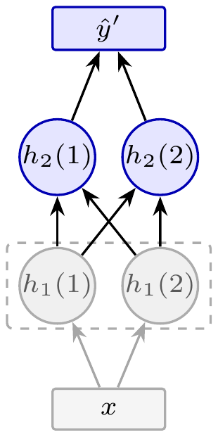
Figure 7.5: Freezing one layer keeps its weights fixed while the rest of the network trains.

Freezing¹²¹²Wikipedia: Fine-tuning (deep learning). keeps selected parameters fixed during training, as in Fig. 7.5. The frozen neurons still compute their values in the forward pass, but their parameters are excluded from the gradient updates. This is a deliberate restriction on what the optimizer is allowed to change.

Freezing is a useful technique to enable transfer learning¹³¹³Freezing is not the same as transfer learning; it is one common tool used when reusing a pretrained network for a new task.. Transfer learning is to reuse part of a network trained on one task for a related new task. A typical workflow is:

1. Start from a network already trained on a large source data set.
2. Keep its lower layers, because they often capture generic features.
3. Add (or replace) an output layer for the new task.
4. Train only this last layer.
5. Optionally unfreeze some of the lower layers and continue training with small learning rate. This is known as fine-tuning.

Thus, by freezing the lower layers we can save computation and protect against overfitting when the new data set is small.

Besides specifying the number and width of the layers, we must consider other aspects of a neural network: which activation functions to use, how many outputs the network should produce, and how information should flow¹⁴¹⁴That is, how the neurons and the layers are connected. between distant parts of the network.

A first question is what a given architecture can represent at all. The universal approximation theorem¹⁵¹⁵Wikipedia: Universal approximation theorem. gives an interesting answer: a one-hidden-layer network suffices, provided it is sufficiently wide, in the following sense. Take a network with one hidden layer (so \(L=2\)) and an identity output activation; then the network computes

\begin{align*} \hat f(x) = \sum_{j=1}^{q_1} A_2(1,j)\, \sigma\rb{\sum_{k=1}^{p} A_1(j,k)\,x(k) + b_1(j)} + b_2, \end{align*}

i.e., a weighted sum of \(q_1\) shifted and stretched copies of the sigmoid function. The theorem says that for every continuous \(f\) on a compact domain and every \(\epsilon>0\) there are a width \(q_1\) and parameters \(A_1,b_1,A_2,b_2\) such that \(|\hat f(x)-f(x)|<\epsilon\) for all \(x\) in that domain. Thus, one hidden layer suffices, provided it is wide enough.

This is an existence result, not a guarantee about training. So the interesting question is not whether an architecture can represent a function, but which architectures reach a given accuracy with few parameters and can still be trained; this is the subject of current research.

Activation functions need not be sigmoid. Another common hidden-layer choice is the ReLU,¹⁶¹⁶Wikipedia: Rectified linear unit.

\begin{align*} \phi(z)&=\max\set{0,z} & \phi'(0) &=0. \end{align*}

This is useful because an active¹⁷¹⁷That is, when \(z>0\). ReLU has derivative \(1\): it passes the gradient backward without shrinking it. A sigmoid hidden unit, by contrast, has derivative at most¹⁸¹⁸\(\sigma'(z)=\sigma(z)\rb{1-\sigma(z)}\leq 1/4\) \(1/4\) and becomes almost flat for large positive or negative \(z\) which leads to the following problem. Recall the backpropagation recursion applied to the simple three-layer feedforward network above. For instance, the derivation in (7.2.2)--(7.2.4) shows that

\begin{align*} \delta_{1} = a_{2} a_{3}\phi_{2}'(z_{2}) \frac{\partial \lscr}{\partial \hat y} \sigma'(z_{3}). \tag{7.3.1} \end{align*}

Each extra layer contributes one more weight and one more slope. So in a stack of, say, \(15\) sigmoid layers the slopes alone contribute a factor of at most \((1/4)^{15}\approx 10^{-9}\). Thus, when using sigmoids throughout, the the small activation derivatives can strongly attenuate gradients through many layers unless the weights compensate, leaving lower layers to learn slowly. This phenomenon is known as vanishing gradients.

ReLU does not suffer from this problem because its derivative is either 0 or 1.¹⁹¹⁹The probability that a preactivation hits 0 is negligible.

A smooth variant of the ReLU is the GELU,²⁰²⁰The Gaussian error linear unit, Wikipedia: Rectified linear unit, GELU. It is used in GPT-style language models.

\begin{align*} \phi(z)=z\,\P{Z\leq z},\qquad Z\sim\Norm{0,1}. \end{align*}

For large positive \(z\) it behaves like the identity and for large negative \(z\) it tends to \(0\), as the ReLU does. It differs near the origin: the GELU is negative for every \(z<0\), with a minimum of about \(-0.17\) at \(z\approx-0.75\), so unlike the ReLU it is not monotone.

Output heads²¹²¹Do not confuse these output heads with the attention heads used inside Transformer layers of large language models. are final output neurons, or final small output layers, for separate prediction tasks, see Fig. 7.6. So far, the network had just one output head: one \(\hat y\) for the input \(x\). However, often we can ask several related questions about the same input. For instance, does a patient have illness A and illness B? Each such question can be answered by its own head but, as Fig. 7.6 shows, all heads share the last hidden layer, \(h_{L-1}\).

For \(K\) such questions, take as logits and outputs

\begin{align*} z^{(r)} = b^{(r)}_{0} + \sum_{j=1}^{q_{L-1}} a^{(r)}(j) h_{L-1}(j), \qquad \hat y^{(r)} = \sigma(z^{(r)}), \qquad r=1,\ldots,K. \end{align*}

Thus, each head has its own training parameters.

⊕
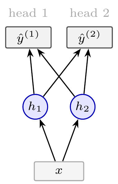
Figure 7.6: Each head is a separate output neuron reading the same hidden layer.

For training, this means that, instead of samples with an outcome \(y\), each observation has multiple targets \(y^{(1)},\ldots,y^{(K)}\), one for each supervised head. Training changes little: take as loss the sum of the \(K\) per-head losses and apply backpropagation as before.

Sharing information from lower layers is efficient: the features \(h_{L-1}(j)\) are learned once but used \(K\) times. Training on multiple labels per input is known as multi-task learning. Because the heads share the hidden layers, the gradient of the summed loss combines contributions from all tasks when updating those layers. If tasks share useful structure, this can encourage a representation that works across tasks and may improve generalization. If their requirements conflict, however, they can interfere.

Skip connections become important in deep networks. A skip connection lets a layer pass its input directly to a later layer. A residual connection²²²²Wikipedia: Residual neural network. is the additive case of a skip connection: the skipped input and the learned update are merged by addition, not by a more general function. The formula below assumes consecutive hidden layers have the same width, so the addition is dimensionally valid; if their widths differ, the skip path needs a projection. So, instead of setting \(h_i = \phi_i(z_i)\) as in (7.2.1), the hidden values are given by

\begin{align*} h_i = h_{i-1} + \phi_i(z_i), \qquad z_i = A_i h_{i-1}+b_i, \end{align*}

equivalently, \(\Delta h_i := h_i-h_{i-1} = \phi_i(z_i)\). Thus, in the forward pass, layer \(i\) adds the update \(\Delta h_i\) to the previous hidden vector.²³²³This is close to an Euler step for a differential equation, where a new state is the old state plus a small change.

⊕
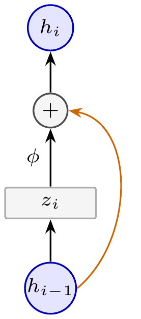
Figure 7.7: A residual connection sends a layer input directly to an addition node, where it is added to the layer update.

The effect of this change on training appears when we differentiate it: the derivative through the layer is

\begin{align*} \frac{\partial h_i}{\partial h_{i-1}} = I + \diag(\phi_i'(z_i))A_i, \end{align*}

and the identity matrix \(I\) provides a direct path for the gradient back to earlier layers. This can help mitigate vanishing gradients, though it does not guarantee that gradients remain large at every layer, as they can still shrink or grow through the learned part of the network.

Residual connections help make networks of dozens or even hundreds of layers trainable. The first famous example was ResNet, an image-recognition network with residual blocks and over a hundred layers; the transformer blocks of large language models also wrap each sublayer in a residual connection.²⁴²⁴Wikipedia: Residual neural network. Wikipedia: Transformer (deep learning architecture). Wikipedia: GPT-3. They also make each layer’s job easier: the layer only needs to learn a small correction to the identity map, not the whole transformation.

A skip connection need not skip just one layer. Examples include ResNet blocks, long U-Net connections, and DenseNet-style dense connections.²⁵²⁵Wikipedia: Residual neural network, which also covers DenseNet. Wikipedia: U-Net.