5 Gradient Descent and Gradient Boosting

The aim of this section is to understand the geometric intuition behind the gradient. This will directly explain why gradient-descent is a natural way to find local minima. We first consider an ordinary function from \(\R\) to \(\R\). We then extend the argument to higher dimensions using paths and the chain rule.

The main idea is simple: To make a function smaller, move in a direction in which its derivative is negative.

Let \(g:\R\longrightarrow\R\) be differentiable, and suppose that we are currently at \(t\). On the real line there are only two possible directions to make \(g\) smaller: left and right. The sign of \(g'(t)\) tells us which way the function increases locally:

• if \(g'(t)>0\), then \(g\) increases when we move to the right, so we should move to the left;
• if \(g'(t)<0\), then \(g\) decreases when we move to the right, so we should move to the right.

Both cases are described by moving in the direction opposite to \(g'(t)\).

To use this to find a local minimum of \(g\), choose a step size \(0 < \eta \ll 1\). Then Taylor’s formula gives

\begin{align*} g(t+\delta)=g(t)+g'(t)\delta+o(\abs{\delta}). \end{align*}

Substituting \(\delta=-\eta g'(t)\), we obtain

\begin{align*} g\rb{t+\delta} &=g(t)-\eta\rb{g'(t)}^2+o(\eta). \end{align*}

If \(g'(t)\neq 0\), the first-order change[fn: That is, the term with \(\eta\).] is strictly negative. Therefore, for sufficiently small \(\eta>0\), \(g\rb{t+\delta}<g(t)\). Thus \(-g'(t)\) gives a local descent direction.

This produces the gradient-descent sequence in one dimension. Starting at \(t^{(0)}\), fix a step size \(\eta>0\) and iterate

\begin{align*} t^{(k+1)}=t^{(k)}-\eta g'\rb{t^{(k)}}. \end{align*}

At an iterate with \(g'(t^{(k)})\neq 0\), if the fixed \(\eta\) is sufficiently small, the update decreases \(g\). If \(g'(t^{(k)})=0\), the update makes no change, and a stationary point need not be a local minimum.²²The Taylor argument shows local decrease, but does not guarantee that one fixed step size decreases \(g\) at every iterate or that the sequence converges to a local minimum. Such claims require additional assumptions on \(g\) and the step size. The Wikipedia article on gradient descent discusses some of its convergence limitations.

Now consider two dimensions. Let \(f:\R^2\longrightarrow\R\) be differentiable. In two dimensions there are infinitely many directions in which \(f\) can change, not just left and right. We must therefore first specify how we move through the domain of \(f\). Let a differentiable path \(\gamma: t \to \gamma(t) \in \R^{2}\) and its derivative with respect to time³³The speed along the path. be given by

\begin{align*} \gamma(t) &= \begin{pmatrix} x(t)\\ y(t) \end{pmatrix}, & \gamma'(t) &= \begin{pmatrix} \dot{x}(t)\\ \dot{y}(t) \end{pmatrix}, \end{align*}

where \(\dot x(t) = \d x(t)/\d t\) and \(\dot y(t) = \d y(t)/\d t\). To keep the notation light below, we write \(x\), \(y\), \(\dot x\), and \(\dot y\) for their values at time \(t\).

Along the path, define

\begin{align*} g_\gamma(t)=(f\circ\gamma)(t)=f\rb{x,y}. \end{align*}

Although \(f\) has a two-dimensional domain, \(g_\gamma\) is again an ordinary function from \(\R\) to \(\R\). We can therefore ask for its ordinary derivative. Apply the same one-dimensional Taylor formula to \(g_\gamma=f\circ\gamma\), and expand the increment one coordinate at a time:

\begin{align*} g_\gamma\rb{t+\delta} &= f\rb{x(t+\delta),y(t+\delta)}\\ &= f\rb{x(t+\delta),y(t+\delta)}-f\rb{x(t+\delta),y} \\ &\quad + f\rb{x(t+\delta),y}-f\rb{x,y} \\ &\quad + f\rb{x,y}\\ &\stackrel1= \partial_y f\rb{x,y}\dot y \delta \\ &\quad + \partial_x f\rb{x,y} \dot x \delta \\ &\quad +f\rb{x,y} + o(\abs{\delta})\\ &\stackrel2= g_\gamma(t) + \delta \ip{\nabla f\rb{x,y},\gamma'(t)} + o(\abs{\delta}). \end{align*}

Step 1 follows from the change caused by moving in the \(y\)-direction, and the change caused by moving in the \(x\)-direction. Step 2 uses that \(g_\gamma(t) = f(x,y)\) and collects the two partial derivatives in the gradient vector:

\begin{align*} \nabla f\rb{x,y}&= \begin{pmatrix} \partial_x f\rb{x,y}\\ \partial_y f\rb{x,y} \end{pmatrix}. \end{align*}

Finally, since \(g_\gamma(t+\delta) = g_\gamma(t) + g_\gamma'(t) \delta + o(\abs{\delta})\), we see that we can take

\begin{align*} g_\gamma'(t) = \ip{\nabla f\rb{x,y},\gamma'(t)}. \end{align*}

Thus the gradient appears by collecting the two coordinate-wise first-order changes into one vector. Clearly, this analysis carries over to \(\R^{n}\) for \(n\geq 2\).

Suppose that \(\gamma\) is a level curve, that is, along \(\gamma\) the function \(g_{\gamma}\) remains constant: for some \(c\),

\begin{align*} g_{\gamma}(t) = f(x,y)=c. \end{align*}

But then \(g_\gamma'(t)=0\); by the chain rule,

\begin{align*} 0 = g_\gamma'(t)=\ip{\nabla f\rb{x,y},\gamma'(t)}. \end{align*}

Therefore the gradient is orthogonal to the level curves of \(f\). Next, if \(\nabla f\rb{x,y}\neq 0\), choosing \(\gamma' = -\nabla f\rb{x,y}/\norm{\nabla f\rb{x,y}}\) makes the inner product as negative as possible among all \(\gamma'\) with unit length. Thus, among steps of a given length, the step opposite to the gradient gives the largest first-order decrease in \(f\).⁴⁴By the Cauchy-Schwarz inequality.

In general, let \(h\) be some small step in some direction, then, we use Taylor’s formula in \(\R^d\) to see that

\begin{align*} f(x+h)=f(x)+\ip{\nabla f(x),h}+o(\norm{h}). \end{align*}

If we choose \(h=-\eta\nabla f(x)\), then

\begin{align*} f\rb{x-\eta\nabla f(x)} = f(x)-\eta\norm{\nabla f(x)}^2+o(\eta). \end{align*}

If \(\nabla f(x)\neq 0\), this lowers \(f\) for sufficiently small positive \(\eta\). Moreover, just as in the one dimensional case, repeating the step gives

\begin{align*} x^{(k+1)} =x^{(k)}-\eta\nabla f\rb{x^{(k)}}. \end{align*}

This is the multidimensional gradient-descent algorithm.⁵⁵The same proviso as in the one-dimensional case applies. Fig. 5.1 provides an illustration.

⊕
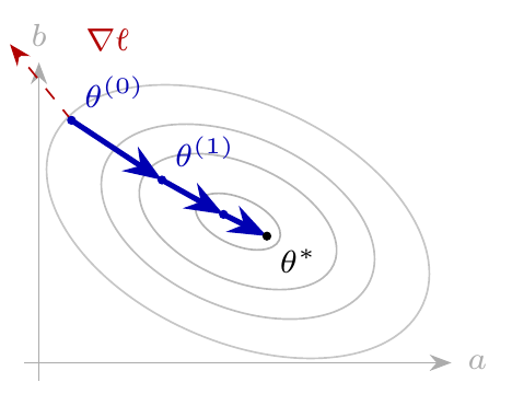
Figure 5.1: Schematic view of gradient descent for \(f:\R^2\to\R\). The arrows move opposite to \(\nabla f\), crossing level curves toward a minimizer.

We can apply the above procedure to the local minimization of \(\hat R_\Tset\). From Taylor’s formula, for a small step \(\Delta\theta\),

\begin{align*} \hat R_{\Tset}(\theta + \Delta\theta) \simeq \hat R_{\Tset}(\theta) + \ip{\nabla\hat R_{\Tset}(\theta), \Delta\theta}. \end{align*}

Then, by the above arguments, for a learning rate \(\eta>0\) that is small enough to keep Taylor’s approximation valid, we have the iterative procedure

\begin{align*} \Delta \theta^{(k)} = - \eta\,\nabla\hat R_{\Tset}(\theta^{(k)}) \end{align*}

from which

\begin{align*} \theta^{(k+1)} &= \theta^{(k)} - \eta \frac{1}{|\Tset|} \sum_{(x,y)\in\Tset} \partial_{2}\lscr\rb{r(y),f_{\theta^{(k)}}(x)}\, \nabla_{\theta}f_{\theta^{(k)}}(x). \tag{5.1.1} \end{align*}

The learning rate needs care. If \(\eta\) is very small, it takes many iterations for the algorithm to converge; if \(\eta\) is too large, the steps overshoot and the iterates may diverge.

\begin{algorithm}
\caption{Gradient descent for a parameterized model class.}
\begin{algorithmic}[1]
\State \textbf{Input:} initial parameters $\theta$, learning rate $\eta>0$, tolerance $\epsilon>0$.
\State \textbf{Output:} parameters $\theta$ with a small gradient.
\Procedure{GradientDescent}{$\theta, \eta, \epsilon$}
    \While{$\norm{\nabla\hat R_{\Tset}(\theta)}^{2} > \epsilon$}
        \State $\theta \gets \theta - \eta\cdot\nabla\hat R_{\Tset}(\theta)$
    \EndWhile
    \Return $\theta$
\EndProcedure
\end{algorithmic}

\end{algorithm}

We close with three remarks. First, (5.1.1) shows a clear pattern: we multiply \(\partial_2 \lscr\) by some correction factor. In gradient boosting below, we will use a similar idea. Second, the gradient is an average over the whole training set, which is expensive when \(\Tset\) is large. Third, a zero gradient does not by itself guarantee a minimum, and where the descent ends can depend on where it starts.

Ordinary least squares is the natural first test of the above rule for \(\theta^{(k)}\). Even though we already know how to solve this with linear algebra, running gradient descent on the same problem shows what the iteration computes.

Recall the model class and the objective (3.2.4). A rule in this class predicts

\begin{align*} \hat y = \beta(x) = \beta_{0} + \ip{\beta, x}, \qquad \beta_{0}\in\R, \quad \beta\in\R^{p}, \end{align*}

so the parameter vector \(\theta = (\beta_{0}, \beta_{1},\ldots,\beta_{p})\) has \(p+1\) components. With squared loss,⁶⁶The factor \(\frac{1}{2}\) changes no minimizer, so every result of Section 3.2.1 still applies; it only removes a factor \(2\) from the derivatives. the loss on a single sample \((x,y)\) is

\begin{align*} \lscr(y, \beta(x)) = \frac{1}{2}\rb{\beta(x)-y}^{2}, \end{align*}

and the training risk is the average of these numbers over the training set,

\begin{align*} \hat R_{\Tset}(\theta) = \frac{1}{2|\Tset|}\sum_{(x,y)\in\Tset}\rb{\beta(x)-y}^{2}. \end{align*}

The partial derivatives follow from the chain rule,⁷⁷\(\partial_{\beta_j} \ip{\beta, x} = x(j)\). applied to one sample at a time:

\begin{align*} \frac{\partial}{\partial \beta_{0}}\lscr(y, \beta(x)) &= \partial_{2}\lscr(y,\beta(x))\, \partial_{\beta_{0}}\beta(x) \\ &= \rb{\beta(x)-y}, \\ \frac{\partial}{\partial \beta_{j}}\lscr(y, \beta(x)) &= \partial_{2}\lscr(y,\beta(x))\, \partial_{\beta_{j}}\beta(x) \\ &= \rb{\beta(x)-y}\,x(j). \end{align*}

The gradient of the training risk is the average of these over \(\Tset\),

\begin{align*} \frac{\partial \hat R_{\Tset}}{\partial \beta_{0}}(\theta) &= \frac{1}{|\Tset|}\sum_{(x,y)\in\Tset}\rb{\beta(x)-y}, \\ \frac{\partial \hat R_{\Tset}}{\partial \beta_{j}}(\theta) &= \frac{1}{|\Tset|}\sum_{(x,y)\in\Tset}\rb{\beta(x)-y}\,x(j), \qquad j = 1,\ldots,p, \end{align*}

and these \(p+1\) numbers together form \(\nabla\hat R_{\Tset}(\theta)\).

The update rule is what we get by inserting these derivatives into (5.1.1). Write \(\theta^{(k)} = (\beta_{0}^{(k)}, \beta_{1}^{(k)}, \ldots, \beta_{p}^{(k)})\) for the parameters after \(k\) steps, and \(\beta^{(k)}(x) = \beta_{0}^{(k)} + \ip{\beta^{(k)}, x}\) for the prediction these parameters make for a feature vector \(x\). Then the step from \(\theta^{(k)}\) to \(\theta^{(k+1)}\) reads

\begin{align*} \beta_{0}^{(k+1)} &= \beta_{0}^{(k)} - \frac{\eta}{|\Tset|} \sum_{(x,y)\in\Tset}\rb{\beta^{(k)}(x) - y}, \\ \beta_{j}^{(k+1)} &= \beta_{j}^{(k)} - \frac{\eta}{|\Tset|} \sum_{(x,y)\in\Tset}\rb{\beta^{(k)}(x) - y}\,x(j), \qquad j = 1,\ldots,p. \tag{5.1.2} \end{align*}

For the intercept, if the current rule predicts too high on average, the sum is positive and \(\beta_{0}\) comes down. For a weight, each sample contributes its prediction error multiplied by its own \(x(j)\), so samples with a large \(j\)th coordinate have more say in \(\beta_{j}\) than samples with a small one, and samples with \(x(j) = 0\) have none at all.

The learning rate can be discussed concretely here. The training risk is quadratic in \(\theta\), so its second-order Taylor expansion is exact. Change only \(\beta_{j}\), by an amount \(\delta\), and keep the other parameters fixed; then⁸⁸\(e_j\) is the unit vector in the \(j\) direction.

\begin{align*} \hat R_{\Tset}(\theta + \delta e_{j}) &= \hat R_{\Tset}(\theta) + \delta\,g_{j} + \frac{1}{2} \delta^{2} s_{j}^{2}, \\ g_{j} &= \frac{\partial \hat R_{\Tset}}{\partial \beta_{j}}(\theta) = \frac{1}{|\Tset|}\sum_{(x,y)\in\Tset}\rb{\beta(x)-y}\,x(j), \\ s_{j}^{2} &= \frac{\partial^{2} \hat R_{\Tset}}{\partial \beta_{j}^{2}}(\theta) =\frac{1}{|\Tset|}\sum_{(x,y)\in\Tset} x(j)^{2}. \end{align*}

Assume \(s_j^2>0\). Along this line the risk is exactly a parabola with curvature \(s_j^2\) and minimum at \(\delta=-g_j/s_j^2\). If \(g_j\neq 0\), the gradient step \(\delta=-\eta g_j\) covers a fraction⁹⁹The ratio of the proposed step to the minimizing step is \((-\eta g_j)/(-g_j/s_j^2)=\eta s_j^2\). \(\eta s_j^2\) of the distance to that minimum: it overshoots when \(\eta>1/s_j^2\) and increases the risk when \(\eta>2/s_j^2\). Thus features with large squared values require smaller steps.

Suppose now that one feature is a distance in meters and another a distance in kilometers. Their values of \(s_{j}^{2}\) can easily differ by a factor \(10^{6}\).

Standardizing the nonconstant features makes each \(s_j^2=1\), removing differences caused by feature scale. However, the calculation considers one coordinate at a time. When all coefficients are updated together, correlations between features also affect the allowable learning rate; standardization does not remove this difficulty.

Probabilities as labels occur whenever the observed value is itself a proportion or a probability, for instance, the fraction of trail that is unpaved. The label space is now \(\Yset=[0,1]\), and the affine rule of the previous section will not do, because \(\beta(x)\) ranges over all of \(\R\) and returns values outside \([0,1]\) for \(|x|\) large.

The repair is to squash the affine score into the unit interval with the sigmoid. We first take a single feature, so that the model has two parameters, and

\begin{align*} \hat y = \sigma(z), \qquad z = \beta(x) = a x + b, \qquad \sigma(z) = \rb{1+e^{-z}}^{-1}, \tag{5.1.3} \end{align*}

with \(\theta = (a,b)\), the weight \(a\) and the bias \(b\). The affine score \(z\) is called the linear predictor or, in the language of neural networks, the logit.

Keeping the squared loss of the previous section, the loss on one sample is

\begin{align*} \lscr(y, f_{\theta}(x)) = \frac{1}{2}\rb{\hat y - y}^{2}, \qquad \hat y = \sigma(\beta(x)). \end{align*}

The partial derivatives now need the chain rule twice, since the parameters reach the loss through \(z\) and then through \(\sigma\). The sigmoid has the convenient derivative

\begin{align*} \sigma'(z) = \sigma(z)\rb{1-\sigma(z)} = \hat y (1-\hat y), \end{align*}

and \(z=ax+b\) contributes \(\partial z/\partial a = x\) and \(\partial z/\partial b = 1\). Multiplying the three factors,

\begin{align*} \frac{\partial}{\partial a}\lscr(y, f_{\theta}(x)) &= \rb{\hat y - y}\, \hat y(1-\hat y)\, x, & \frac{\partial}{\partial b}\lscr(y, f_{\theta}(x)) &= \rb{\hat y - y}\,\hat y(1-\hat y). \end{align*}

Writing \(\beta^{(k)}(x)=a^{(k)}x+b^{(k)}\) and \(\hat y^{(k)}(x)=\sigma(\beta^{(k)}(x))\) for the prediction of the current parameters, the update (5.1.1) becomes

\begin{align*} a^{(k+1)} &= a^{(k)} - \frac{\eta}{|\Tset|}\sum_{(x,y)\in\Tset} \rb{\hat y^{(k)}(x) - y}\,\hat y^{(k)}(x)\rb{1-\hat y^{(k)}(x)}\,x, \\ b^{(k+1)} &= b^{(k)} - \frac{\eta}{|\Tset|}\sum_{(x,y)\in\Tset} \rb{\hat y^{(k)}(x) - y}\,\hat y^{(k)}(x)\rb{1-\hat y^{(k)}(x)}. \tag{5.1.4} \end{align*}

Three things changed with respect to the previous section, and all three come from the sigmoid. First, there is no closed form to fall back on: setting the derivatives to zero gives equations in which \(a\) and \(b\) sit inside \(\sigma\), so they cannot be separated into a linear system. Second, the training risk need no longer be convex in \(\theta\), so the caveat of the introduction becomes relevant: different starting points may end at different fitted parameters.

Third, and most important for what follows, the factor \(\hat y(1-\hat y)\) is at most \(1/4\), and it is near zero exactly when \(\hat y\) is near \(0\) or \(1\). To see the size of this effect, take \(y=0\) and compare two predictions. A hesitant \(\hat y = 0.5\) contributes \(\rb{\hat y - y}\hat y(1-\hat y) = 0.5\cdot 0.25 = 0.125\) per unit of \(x\) to the sum, while a confidently wrong \(\hat y = 0.999\) contributes \(0.999\cdot 0.000999 \approx 0.001\). The sample that is almost maximally wrong therefore moves the parameters more than a hundred times less than the one that is hesitant. The reason is geometric: \(\hat y\) near \(1\) means \(z = ax+b\) lies far from \(0\), where the sigmoid is flat, so changing \(a\) or \(b\) hardly changes \(\hat y\) and hardly changes the loss. This effect is called saturation.

Binary labels are such that \(y\in\set{0,1}\): the trail edge is bad or it is not, the email is spam or it is not. Since \(\set{0,1}\subset[0,1]\), this is not a new label space at all, and the model (5.1.3) can stay exactly as it is. What changes is what we may say about the label. A fraction is a number we simply observe, and the loss that compares it with a prediction is ours to choose. A binary label is the outcome of a draw, and if we are willing to model that draw, then the loss follows from the model instead of being chosen by hand.

So assume that, given the features, the labels are independent, and that the model returns the probability of the outcome \(y=1\),

\begin{align*} \P{Y = 1 \mid x} = \hat y = \sigma(\beta(x)). \end{align*}

Then a sample with \(y=1\) has probability \(\hat y\) and one with \(y=0\) has probability \(1-\hat y\), which the single expression \(\hat y^{y}(1-\hat y)^{1-y}\) covers, so the likelihood of the observed labels is

\begin{align*} L(a,b) = \prod_{(x,y)\in\Tset} \hat y(x)^{\,y}\rb{1-\hat y(x)}^{1-y}. \end{align*}

The parameters that make the observed labels most probable are those that maximize \(L\), and because the logarithm is increasing, they are also the ones that minimize \(-\log L\), and hence \(-\log L/|\Tset|\). This average is the training risk \(\hat R_{\Tset}(a,b)\) when the loss on a single sample is the binary cross-entropy loss,

\begin{align*} \lscr(y, f_{\theta}(x)) = -y\log \hat y - (1-y)\log(1-\hat y). \tag{5.1.5} \end{align*}

The partial derivatives are again a chain rule. Using \(\sigma'(z) = \hat y(1-\hat y)\) once more,

\begin{align*} \frac{\partial}{\partial a}\log \hat y &= \frac{\hat y (1-\hat y)}{\hat y}\frac{\partial z}{\partial a} = (1-\hat y)x, & \frac{\partial}{\partial b}\log \hat y &= 1-\hat y, \end{align*}

and the same calculation for \(\log(1-\hat y)\) gives

\begin{align*} \frac{\partial}{\partial a}\log(1-\hat y) &= -\hat y x, & \frac{\partial}{\partial b}\log(1-\hat y) &= -\hat y. \end{align*}

Hence,

\begin{align*} \frac{\partial}{\partial a}\lscr(y, f_{\theta}(x)) &= -\rb{y(1-\hat y)x - (1-y)\hat y x} = \rb{\hat y - y}x, & \frac{\partial}{\partial b}\lscr(y, f_{\theta}(x)) &= \hat y - y. \end{align*}

The update rule becomes

\begin{align*} a^{(k+1)} &= a^{(k)} - \frac{\eta}{|\Tset|}\sum_{(x,y)\in\Tset} \rb{\hat y^{(k)}(x) - y}\,x, & b^{(k+1)} &= b^{(k)} - \frac{\eta}{|\Tset|}\sum_{(x,y)\in\Tset} \rb{\hat y^{(k)}(x) - y}. \end{align*}

Compare this with (5.1.4): the model is the same, the data are the same, but the factor \(\hat y(1-\hat y)\) has disappeared. The prediction error remains, exactly as it was for OLS. So a confidently wrong prediction produces a large correction, and saturation is gone. Moreover, the training risk under the cross-entropy loss is convex in \(\theta\), so every point with zero gradient is a global minimizer, and the second limitation of the descent step does not apply.

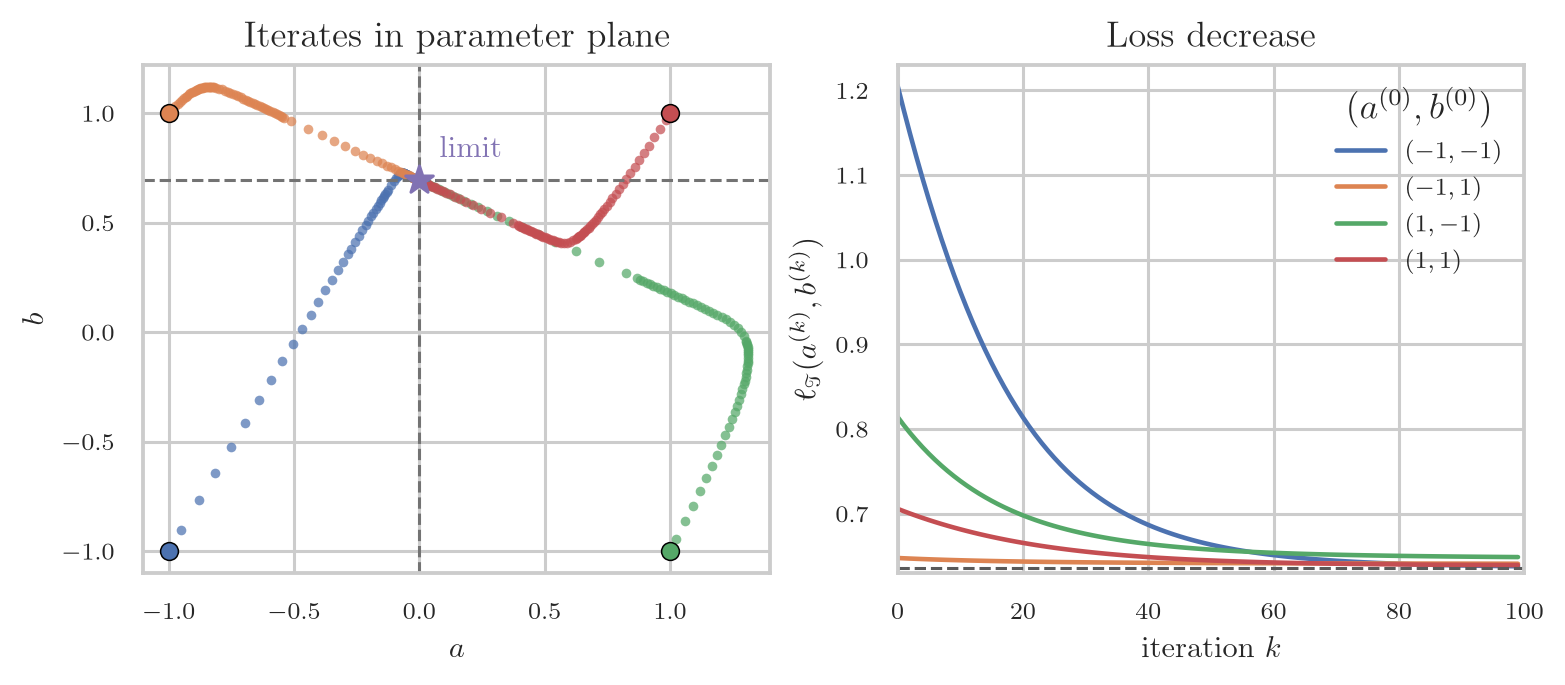
Alg. 5.1.2 collects the steps. Fig. 5.2 shows the paths for four starting points. All four converge to the same limit, and the training risk falls quickly at first while the parameters themselves are still moving slowly.

\begin{algorithm}
\caption{Gradient descent for a sigmoid with binary labels.}
\begin{algorithmic}[1]
\State \textbf{Input:} training set $\Tset$, initial parameters $a,b$, learning rate $\eta>0$, tolerance $\epsilon>0$.
\State \textbf{Output:} parameters $a, b$.
\Procedure{SigmoidGradientDescent}{$\Tset,a,b,\eta,\epsilon$}
    \While{$\norm{\nabla\hat R_{\Tset}(a,b)}^{2} > \epsilon$}
        \State $\hat y_i \gets\sigma(a\cdot x_i+b)$ for every $(x_i,y_i) \in \Tset$.
        \State $\nabla_a \gets \frac{1}{|\Tset|}\sum_{(x_i,y_i)\in\Tset}(\hat y_i-y_i)\cdot x_i$, $\nabla_b \gets \frac{1}{|\Tset|}\sum_{(x_i,y_i)\in\Tset}(\hat y_i-y_i)$.
        \State $a \gets a - \eta\cdot\nabla_a$, $b \gets b - \eta\cdot\nabla_b$.
    \EndWhile
    \Return $(a,b)$
\EndProcedure
\end{algorithmic}

\end{algorithm}

With more features nothing changes except for the bookkeeping. Put \(\beta(x)=\beta_0+\ip{\beta,x}\) and \(\hat y = \sigma(\beta(x))\) for a feature vector \(x\in\R^{p}\), so that

\begin{align*} \frac{\partial}{\partial \beta_{0}}\lscr(y, f_{\theta}(x)) &= \hat y - y, & \frac{\partial}{\partial \beta_{j}}\lscr(y, f_{\theta}(x)) &= \rb{\hat y - y}\,x(j). \end{align*}

This is two-class logistic regression (3.3.10). For \(K\) classes the softmax (3.3.8) takes the place of the sigmoid, and the three steps are once more the same: write the loss of one sample, differentiate it once per parameter, average over the training set.

The cost per step of (5.1.2) is one pass over the entire training set. When the training set is large, this is the dominant cost of fitting, and it has to be paid again at every iteration.

Stochastic gradient descent¹⁰¹⁰Wikipedia: Stochastic approximation. replaces the gradient over the entire set \(\Tset\) in (5.1.1) by the gradient of a single sample \((X,Y)\) drawn uniformly from \(\Tset\). This replacement is unbiased,

\begin{align*} \E{\nabla_{\theta}\lscr(r(Y), f_{\theta}(X))} = \frac{1}{|\Tset|}\sum_{(x,y)\in\Tset}\nabla_{\theta}\lscr(r(y), f_{\theta}(x)) = \nabla\hat R_{\Tset}(\theta), \end{align*}

because a uniform draw gives each of the \(|\Tset|\) samples probability \(1/|\Tset|\), so that the expectation is precisely the average that defines the full gradient. Thus the update \( \theta^{(k+1)} = \theta^{(k)} - \eta\,\left.\nabla_{\theta}\lscr(r(Y), f_{\theta}(X))\right|_{\theta=\theta^{(k)}} \) moves, on expectation, in the same direction as the full gradient descent of (5.1.1). The advantage is that each step is cheap as it uses the gradient of just one sample. The disadvantage is that the sequence of updates is noisy, as each step depends only on the sample that happens to be drawn.

Mini-batching is a compromise often used in practice. Instead of one sample, choose a batch \(\Bset\), a set of samples drawn at random from \(\Tset\) without replacement,¹¹¹¹The batch size controls the tradeoff between cost and noise. There is no universally best size for \(\Bset\). Small \(\Bset\) is cheap but noisy. Large \(\Bset\) is stable, but uses more memory and computation. Sizes are usually powers of two between \(32\) and \(256\). and use the gradient of the empirical risk on that batch,

\begin{align*} \nabla\hat R_{\Bset}(\theta) = \frac{1}{|\Bset|}\sum_{(x,y)\in\Bset}\nabla_{\theta}\lscr(r(y), f_{\theta}(x)), \tag{5.1.6} \end{align*}

as an approximation of the full gradient. By the same argument as for stochastic gradient descent, \(\E{\nabla\hat R_{\Bset}(\theta)}=\nabla\hat R_{\Tset}(\theta)\). Thus mini-batch gradient descent still moves in the correct direction on average, but it is less noisy than pure stochastic gradient descent.

We still want every training sample in \(\Tset\) to contribute to the parameter updates. We do this by splitting the training set \(\Tset\) at random into disjoint batches and using each batch, in turn, to compute the mini-batch gradient in (5.1.6). One training epoch consists of one round in which all batches have been used once. One epoch contains \(\lceil |\Tset|/|\Bset|\rceil\) parameter updates.¹²¹²When \(|\Bset|\) does not divide \(|\Tset|\), the last batch has fewer than \(|\Bset|\) samples.

Reshuffling the samples into new batches at the start of each epoch is important: it prevents the same samples from always appearing together.

Fix a base class \(\Hset\) of prediction functions. Its members are called base learners or weak learners: each is a simple rule that, on its own, predicts only slightly better than guessing. A decision stump, a tree of depth one, is the simplest example.

Boosting is an ensemble method, like bagging, but the ensemble is a sum rather than an average. After \(B\) rounds the prediction function is the additive model

\begin{align*} f_B(x) = f_0(x) + \eta\sum_{b=1}^{B} \rho_b\, h_b(x), \end{align*}

with base learners \(h_b \in \Hset\), coefficients \(\rho_b \in \R\), a learning rate \(\eta > 0\), and a starting function \(f_0\). Each \(h_b\) is simple, but the sum \(f_B\) need not be: with stumps as base learners and a single feature, \(f_B\) is a step function with up to \(B\) jumps.

For fixed \(f_0\) and \(\eta\), the model class of Chapter 3 consists of all sums of the displayed form, obtained by choosing the base learners \(h_b\) and coefficients \(\rho_b\). Increasing \(B\) enlarges this class and can permit a closer fit to the training data.

Boosting happens forward stagewise: at round \(b\) it holds \(f_{b-1}\) fixed and then asks for the pair \((h_b, \rho_b)\) that lowers the training risk \(\hat R_\Tset\) most:

\begin{align*} (h_b, \rho_b) = \argmin_{h \in \Hset,\, \rho \in \R} \frac{1}{|\Tset|}\sum_{(x,y) \in \Tset} \lscr\rb{y, f_{b-1}(x) + \rho\, h(x)}. \tag{5.2.1} \end{align*}

Then it uses this pair to update

\begin{align*} f_b(x) = f_{b-1}(x) + \eta\, \rho_b\, h_b(x). \tag{5.2.2} \end{align*}

Once a term has been added it is never revisited. Each round is therefore one small fitting problem instead of a joint search over \(B\) base learners at once. It also makes boosting greedy: nothing guarantees that \(f_B\) is the best sum of \(B\) members of \(\Hset\).

The learning rate \(\eta\) scales every correction; with smaller \(\eta\) more rounds are needed to reach the same fit.

Any class \(\Hset\) can be used in principle, but shallow regression trees are the usual choice. A tree splits on the features themselves and can capture non-linear behavior. Second, fitting a tree of small depth is fast, which matters when the fit is repeated \(B\) times. Third, shallow trees have low variance. The problem that a single weak learner is highly biased is mitigated by forming an ensemble.

Gradient boosting is a three step approach to approximate (5.2.1). For a small correction function \(h\in \Hset\), Taylor’s formula gives¹⁴¹⁴Here \(\partial_2\lscr(y,a)\) denotes the partial derivative of the loss with respect to its second argument \(a\), while the label \(y\) is held fixed.

\begin{align*} \hat R_{\Tset}(f+h) &=\frac{1}{|\Tset|}\sum_{(x,y)\in\Tset} \lscr\rb{y,f(x)+h(x)}\\ &=\frac{1}{|\Tset|}\sum_{(x,y)\in\Tset} \qb{\lscr\rb{y,f(x)} +\partial_2\lscr\rb{y,f(x)}h(x)+\cdots}\\ &=\hat R_{\Tset}(f) +\frac{1}{|\Tset|}\sum_{(x,y)\in\Tset} \partial_2\lscr\rb{y,f(x)}h(x)+\cdots. \end{align*}

Thus, to decrease the risk, \(h(x)\) should have the opposite sign to \(\partial_2\lscr\rb{y,f(x)}\) on each sample \((x,y)\in\Tset\).

We cannot generally choose the values \(h(x_i)\) independently, because \(h\in\Hset\) imposes a constraint on the possible corrections. We choose a base learner whose predictions approximate the negative derivatives as closely as possible in squared error:

\begin{align*} h^*=\argmin_{h\in\Hset} \frac{1}{2}\sum_{i=1}^{|\Tset|}\rb{\rscr_i-h(x_i)}^2, \tag{5.2.3} \end{align*}

where the pseudo-residuals are defined as,

\begin{align*} \rscr_i=-\partial_2\lscr\rb{y_i,f(x_i)}. \tag{5.2.4} \end{align*}

Thus \(h^*\) is the closest approximation, within the base class, to the negative gradient at the training samples.¹⁵¹⁵The square loss here is only a convenient projection loss for fitting the pseudo-residuals. It is not the original prediction loss \(\lscr\), which is the loss minimized by the line search below.

The line search then determines how far to move along this fitted direction:

\begin{align*} \rho^*&=\argmin_{\rho\in\R} \hat R_{\Tset}\rb{f+\rho h^*}\\ &=\argmin_{\rho\in\R}\frac{1}{|\Tset|} \sum_{(x,y)\in\Tset} \lscr\rb{y,f(x)+\rho h^*(x)}. \tag{5.2.5} \end{align*}

Observing that the argument above applies to every current prediction function \(f\), we can use this to turn it into an iterative procedure. Start with the constant function (5.2.6)

\begin{align*} f_0(x) = c^{*} = \argmin_{c \in \R} \sum_{(x,y)\in\Tset} \lscr\rb{y,c}. \tag{5.2.6} \end{align*}

Suppose now that round \(b\) starts with \(f_{b-1}\). Apply the preceding argument with \(f=f_{b-1}\). This gives the pseudo-residuals \(\rscr_i^{(b)}\), the fitted base learner \(h_b\), and the line-search coefficient \(\rho_b\) by exactly the three steps described above. We then update the predictor to \(f_b=f_{b-1}+\eta\rho_b h_b\). Therefore the generic \(f\mapsto h^*\mapsto\rho^*\) argument is repeated with the newly obtained \(f_b\) at the next round. The algorithm below collects exactly these steps for \(b=1,\ldots,B\).

\begin{algorithm}
\caption{Gradient boosting for a differentiable loss \(\lscr\).}
\begin{algorithmic}[1]
\State \textbf{Input:} a training set $\Tset$, a base class $\Hset$, the number $B$ of rounds, a learning rate $\eta > 0$.
\State \textbf{Output:} a prediction function $f_B$.
\Procedure{GradientBoost}{$\Tset, \Hset, B, \eta$}
    \State $f_{0} \gets \argmin_{c \in \R} \sum_{(x,y) \in \Tset} \lscr(y, c)$.
    \For{$b = 1, \ldots, B$}
        \State $\rscr_i^{(b)} \gets -\left.\partial_2\lscr(y_i, a)\right|_{a = f_{b-1}(x_i)}$ for all $i$ \Comment{Negative gradient.}
        \State $h_b \gets \argmin_{h \in \Hset} \sum_{i} \rb{\rscr_i^{(b)} - h(x_i)}^{2}$ \Comment{Fit a base learner.}
        \State $\rho_b \gets \argmin_{\rho \in \R} \sum_{(x,y)\in\Tset} \lscr\rb{y, f_{b-1}(x) + \rho\cdot h_b(x)}$ \Comment{Line search.}
        \State $f_b \gets f_{b-1} + \eta\cdot\rho_b\cdot h_b$
    \EndFor
    \Return $f_B$
\EndProcedure
\end{algorithmic}

\end{algorithm}

We next apply gradient boosting to a regression and a classification problem.

Take the regression setting of Section 3.2.1, \(\Yset = \Aset = \R\), with the loss

\begin{align*} \lscr(y, a) = \frac{1}{2} (y-a)^{2}. \end{align*}

The initialization (5.2.6) is the constant that minimizes \(\sum_{(x,y)\in\Tset}(y-c)^{2}\), which is the sample mean \(\bar y\), as derived in Section 3.2.1. Next, \(-\partial_2\lscr(y,a) = y - a\), so (5.2.4) gives

\begin{align*} \rscr_i^{(b)} = y_i - f_{b-1}(x_i). \end{align*}

The first residuals \(\rscr_i^{(1)} = y_i - \bar y\) are the part of each label that a single constant cannot explain. Fit a shallow regression tree \(h_1\) to the pairs \((x_i, \rscr_i^{(1)})\); by (5.2.3) this is an ordinary least-squares tree fit with the residuals as labels. Below we show that the line search gives \(\rho_b=1\). Thus, it suffices to add a fraction \(\eta\) of this tree to the constant, recompute the residuals \(\rscr_i^{(2)} = y_i - f_1(x_i)\), fit the next tree to those, and so on; we have all ingredients to operate Alg. 5.2.1.

To see that the line search gives \(\rho_b =1\), use \(\rscr_i^{(b)} = y_i - f_{b-1}(x_i)\) to write the objective of (5.2.5) as \(\frac{1}{2}\sum_i (\rscr_i^{(b)} - \rho h_b(x_i))^{2}\), set its derivative with respect to \(\rho\) to zero, and simplify:¹⁶¹⁶Provided \(\sum_i h_b(x_i)^{2} > 0\); a tree with all leaf values zero adds nothing.

\begin{align*} \rho_b = \frac{\sum_i \rscr_i^{(b)} h_b(x_i)}{\sum_i h_b(x_i)^{2}}. \end{align*}

Write \(\set{\Tset_1, \ldots, \Tset_m}\) for the partition of the training samples formed by the leaves of \(h_b\), as in (4.1.1), and \(c_t\) for the value stored in leaf \(t\). A least-squares regression tree stores in each leaf the mean of the values it was fitted on, so \(c_t=|\Tset_t|^{-1}\sum_{i \in \Tset_t} \rscr_i^{(b)}\), hence \(\sum_{i\in\Tset_t} \rscr_i^{(b)}=|\Tset_t| c_t\). Summing over the leaves,

\begin{align*} \sum_i \rscr_i^{(b)} h_b(x_i) = \sum_{t=1}^{m} c_t \sum_{i \in \Tset_t} \rscr_i^{(b)} = \sum_{t=1}^{m} |\Tset_t| c_t^{2} = \sum_i h_b(x_i)^{2}. \end{align*}

By using this in the expression for \(\rho_b\), it follows that \(\rho_b=1\).

Interestingly, with a convenient choice for \(\eta\), we can see that the sum over the squared residuals decrease for every step. Since \(\rho_b = 1\), the update (5.2.2) replaces each \(\rscr_{i}^{(b)}\) by \(\rscr_{i}^{(b)} - \eta c_t\), which turns the sum of squares on leaf \(t\) into

\begin{align*} \sum_{i\in \Tset_t} (\rscr_{i}^{(b)} - \eta c_t)^{2} & = \sum_{i\in \Tset_t} (\rscr_{i}^{(b)})^{2} - 2\eta c_t \sum_{i\in \Tset_t}\rscr_{i}^{(b)} + |\Tset_t|\,\eta^{2}c_t^{2} \\ & = \sum_{i\in \Tset_t} (\rscr_{i}^{(b)})^{2} - \eta(2-\eta)\,|\Tset_t|\,c_t^{2}. \end{align*}

Since \(\eta(2-\eta) > 0\) for every¹⁷¹⁷This covers the small \(\eta\) used in practice. \(\eta\in(0,2)\) the decrease is strict on a leaf whose mean residual is nonzero. Summing over all leaves in the partition shows that the sum over the squared residuals becomes smaller.

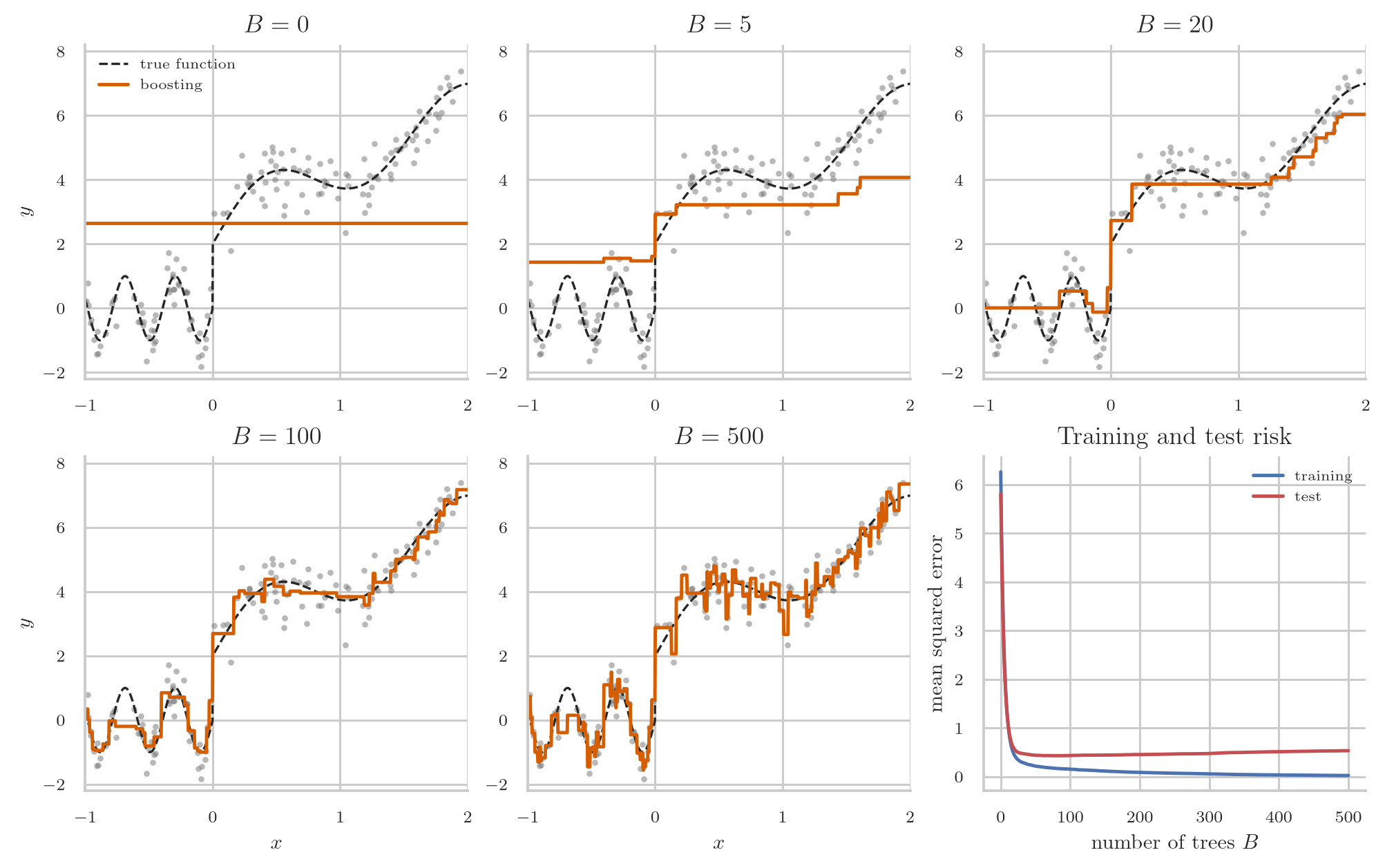
The training risk therefore keeps falling as trees are added, but the validation risk typically does not. At first the added learners pick up structure that the earlier ones missed and the validation risk falls with the training risk, but after enough rounds the added trees fit the training samples only, and the validation risk rises again. Fig. 5.3 provides an example.

We will show how the steps of gradient boosting can be applied to classification. This is known as AdaBoost.¹⁸¹⁸Wikipedia: AdaBoost. Wikipedia: XGBoost is an implementation of gradient tree boosting.

Take binary classification with¹⁹¹⁹The two labels are a relabeling of the \(\set{0,1}\) convention used elsewhere in the book. The point of the relabeling is that below the sign of \(y f(x)\) tells whether a prediction is correct, and \(y h(x) \in \set{-1, 1}\) for a base learner \(h\).

\begin{align*} \Yset = \set{-1, +1}, \qquad \Aset = \R. \end{align*}

The prediction \(f(x)\in\R\) is a score, and the decision map of (3.1.1) is

\begin{align*} \hat y = d(f(x)) = \sign(f(x)). \end{align*}

Here we use the convention \(\sign(0)=+1\), so a zero score predicts \(+1\). The quantity

\begin{align*} y f(x) \end{align*}

is the margin of the sample \((x,y)\). It is positive when the sign of the score matches the label, so the classification is correct, and negative when it does not.

The base class is a set of stumps that map to \(\set{-1, 1}\),

\begin{align*} \Hset \subset \set{h : \Xset \to \set{-1, +1}}. \end{align*}

To compute the pseudo residuals, the derivative of the loss should be meaningful. Zero-one loss is \(\1{y \neq d(f(x))}\). As a function of the score, it has derivative zero wherever it is differentiable, so its derivative gives no useful direction for gradient-based fitting. AdaBoost replaces this loss by the exponential loss

\begin{align*} \lscr(y, a) = e^{-y a}, \tag{5.2.7} \end{align*}

which is differentiable, decreasing in the margin, and satisfies \(\1{y\neq d(a)}\le e^{-ya}\) for all labels \(y\in\set{-1,+1}\) and scores \(a\in\R\). The training risk under exponential loss is therefore an upper bound for the misclassification rate. Minimizing it minimizes a smooth upper bound, although the misclassification rate need not decrease at every iteration.

Differentiating (5.2.7) gives \(\partial_2\lscr(y,a) = -y e^{-ya}\), so (5.2.4) reads

\begin{align*} \rscr_i^{(b)} = y_i \tilde w_i^{(b)}, \qquad \tilde w_i^{(b)} := e^{-y_i f_{b-1}(x_i)}. \tag{5.2.8} \end{align*}

Thus the pseudo-residual of sample \(i\) factors into a label and a positive number \(\tilde w_i^{(b)}\) that depends only on the margin. A sample with a large positive margin has \(\tilde w_i^{(b)}\) close to \(0\); a misclassified sample has margin below \(0\) and hence \(\tilde w_i^{(b)} > 1\). By normalizing

\begin{align*} w_i^{(b)} = \frac{\tilde w_i^{(b)}}{\sum_{j=1}^{|\Tset|} \tilde w_j^{(b)}}, \qquad \sum_{i=1}^{|\Tset|} w_i^{(b)} = 1, \tag{5.2.9} \end{align*}

\(w^{(b)}\) becomes a probability vector over the training samples.

For a vector of scores \(s\in\R^m\), the softmax function \(\sm\) in (3.3.8) turns them into a probability vector, with larger scores giving larger probabilities. The normalization (5.2.9) is exactly this softmax function: \(w^{(b)} = \sm(s^{(b)})\) with scores \(s_i^{(b)} = -y_i f_{b-1}(x_i)\), the negated margins. Here the index runs over the \(|\Tset|\) training samples, so the softmax produces a pmf over samples; in classification it runs over the classes instead.

The next step in gradient boosting is the square loss optimization over \(h_b\). Substitute (5.2.8) into the fitting step (5.2.3) and expand the square:

\begin{align*} \frac{1}{2}\sum_{i=1}^{|\Tset|} \rb{\rscr_i^{(b)} - h(x_i)}^{2} = \frac{1}{2}\sum_{i=1}^{|\Tset|} \rb{\rscr_i^{(b)}}^{2} - \sum_{i=1}^{|\Tset|} \rscr_i^{(b)} h(x_i) + \frac{1}{2}\sum_{i=1}^{|\Tset|} h(x_i)^{2}. \end{align*}

The first term does not involve \(h\). The third equals \(|\Tset|/2\), because \(h(x_i)^{2}=1\) for every \(h \in \Hset\). Therefore,

\begin{align*} \argmin_{h\in \Hset}\sum_i \rb{\rscr_i^{(b)} - h(x_i)}^{2} = \argmax_{h\in \Hset} \sum_i \tilde w_i^{(b)} y_i h(x_i). \end{align*}

Rewriting this sum in terms of the misclassified samples prepares the line search over \(\rho_b\). Since \(y_i\) and \(h(x_i)\) both lie in \(\set{-1,+1}\),

\begin{align*} y_i h(x_i) = 1 - 2\cdot\1{y_i \neq h(x_i)}, \end{align*}

so that, dividing by the positive constant \(\sum_j \tilde w_j^{(b)}\),

\begin{align*} \frac{\sum_i \tilde w_i^{(b)} y_i h(x_i)}{\sum_j \tilde w_j^{(b)}} = 1 - 2 \err_{b}(h), \end{align*}

where the weighted misclassification error is given by

\begin{align*} \err_b(h) = \sum_{i=1}^{|\Tset|} w_i^{(b)} \1{y_i \neq h(x_i)}. \tag{5.2.10} \end{align*}

With this, the fitting step (5.2.3) becomes

\begin{align*} h_b = \argmin_{h \in \Hset} \err_b(h). \tag{5.2.11} \end{align*}

The line search has a simple solution.

Proof

For the line search (5.2.5)

\begin{align*} \argmin_{\rho \in \R} \sum_{i} \lscr\rb{y_i, f_{b-1}(x_i) + \rho h_b(x_i)} \end{align*}

split the sum by whether \(h_b\) classifies sample \(i\) correctly, using \(y_i h_b(x_i) = \pm 1\):

\begin{align*} \sum_{i=1}^{|\Tset|} e^{-y_i (f_{b-1}(x_i) + \rho h_b(x_i))} &= \sum_{i=1}^{|\Tset|} \tilde w_i^{(b)} e^{-\rho y_i h_b(x_i)} \\ & = e^{-\rho} \sum_{i=1}^{|\Tset|} \tilde w_i^{(b)} \1{y_{i} = h_{b}(x_{i})} + e^{\rho} \sum_{i=1}^{|\Tset|} \tilde w_i^{(b)} \1{y_{i} \neq h_{b}(x_{i})}. \end{align*}

Dividing by \(\sum_j \tilde w_j^{(b)}\) leaves the minimizer unchanged and replaces \(\tilde w\) by \(w\). With (5.2.10) the two sums become \(1-\err_b(h_b)\) and \(\err_b(h_b)\), so we must minimize

\begin{align*} G(\rho) = e^{-\rho}(1-\err_b(h_b)) + e^{\rho}\err_b(h_b). \tag{5.2.13} \end{align*}

This is a function of one variable with \(G''(\rho) = e^{-\rho}(1-\err_b(h_b)) + e^{\rho}\err_b(h_b) > 0\) whenever \(0 < \err_b(h_b) < 1\), hence strictly convex, so the stationary point is the minimum. From \(G'(\rho) = -e^{-\rho}(1-\err_b(h_b)) + e^{\rho}\err_b(h_b) = 0\) and solving for \(\rho_{b}\) the result follows.

A classifier with \(0<\err_b(h_b)<1/2\) guesses better than random and gets \(\rho_b>0\); one that guesses, \(\err_b(h_b) = 1/2\), gets \(\rho_b = 0\) and is not added at all.²¹²¹When \(\err_b(h_b) > 1/2\), use \(-h_b\) as the improvement. The requirement \(\err_b(h_b) < 1/2\) is known as the weak-learning condition.

Observe that in the above we used the weights \(w^{(b)}\), which in turn depend on \(f_{b-1}\) through (5.2.9). Once we have the update \(h_b\), we need to update these weights for the next iteration. Using the update (5.2.2),

\begin{align*} \tilde w_i^{(b+1)} = e^{-y_i f_b(x_i)} = e^{-y_i f_{b-1}(x_i)} e^{-\eta \rho_b y_i h_b(x_i)} = \tilde w_i^{(b)} e^{-\eta \rho_b y_i h_b(x_i)}, \end{align*}

and after normalizing,

\begin{align*} w_i^{(b+1)} = \frac{w_i^{(b)} e^{-\eta \rho_b y_i h_b(x_i)}} {\sum_{j=1}^{|\Tset|} w_j^{(b)} e^{-\eta \rho_b y_j h_b(x_j)}}. \tag{5.2.14} \end{align*}

Since \(y_i h_b(x_i) = \pm 1\), the numerator multiplies \(w_i^{(b)}\) by \(e^{-\eta\rho_b} < 1\) when sample \(i\) is classified correctly and by \(e^{\eta\rho_b} > 1\) when it is not. Samples that the new classifier gets wrong gain weight, and by (5.2.11) the next classifier is chosen to do better on exactly those samples.

For the initialization (5.2.6), let \(n_+\) and \(n_-\) count the samples with \(y_i = +1\) and \(y_i = -1\), and assume both classes occur, so \(n_+>0\) and \(n_->0\). Then \(\sum_{(x,y)\in\Tset} e^{-y c} = n_+ e^{-c} + n_- e^{c}\), and setting its derivative to zero gives \(f_0(x) = \frac12 \log(n_+/n_-)\). AdaBoost as usually stated takes \(f_0 = 0\) instead, which by (5.2.9) starts the weights uniform at \(w_i^{(1)} = 1/|\Tset|\), and takes \(\eta=1\), so that each classifier enters with its full coefficient \(\rho_b\).

Fig. 5.4 shows an example of AdaBoost.

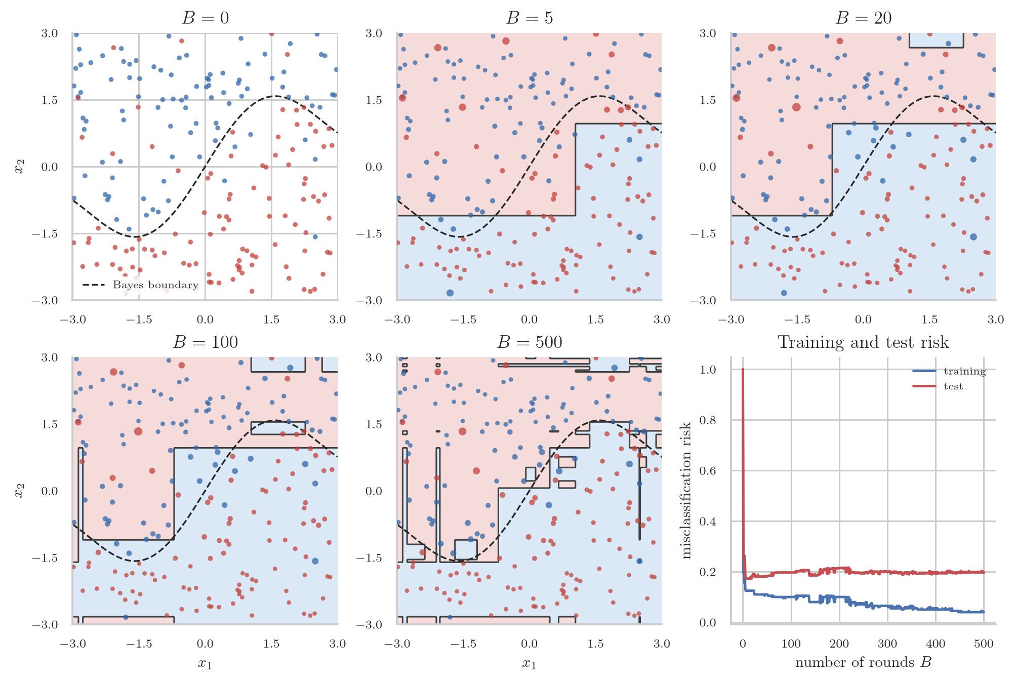
We remark in passing that it can be shown that with \(\eta=1\), if \(\err_b(h_b) \le 1/2 - \gamma\) for some fixed \(\gamma > 0\) and all \(b\), then the training risk of \(\sign(f_B)\) under zero-one loss is at most \(e^{-2\gamma^{2}B}\). Thus, the bound falls geometrically in \(B\). Consequently, classifiers that are each only slightly better than guessing can drive the training error to zero. Thus, the training risk cannot be used to choose \(B\); use the validation risk as in Section 3.6.