
1.4 Fighting the Exponential Distribution is Futile
1.4 Fighting the Exponential Distribution is Futile
Perhaps the mathematical arguments in the preceding section have not fully convinced you that exponential inter-arrival times and Poisson arrival counts arise naturally in many systems. We therefore use a simulation to show how exponential inter-arrival times emerge when many nearly periodic patient streams are combined.
The simulation is based on an internship of one of my master’s students with the task of evaluating the scheduling system for patients with inflammatory bowel disease (IBD) at a hospital. Patients with IBD can be categorized as regular and urgent. Regular patients required check-ups approximately every six months, whereas urgent patients needed to be seen within one week, that is, five working days.1This procedure has been changed recently; however, the ideas of this case apply much more generally. Each consultation takes 10 minutes. Immediately after a consultation, regular patients scheduled their next visit for approximately six months later. There are about 1000 patients in the system and a working year consists of 200 working days. Given that each patient is seen twice per year, a physician needed to consult with an average of 10 patients daily.2Two visits per year per patient times 1000 patients distributed over 200 days per year is 10 patients per day. The problem was to design a planning procedure that allowed enough flexibility to meet the time constraints for the urgent patients without leading to idle times for the physicians. Of course, new patient intakes occurred, but for simplicity we assume that the patient population remains constant.
Planning regular patients six months in advance seems to lead to stable arrival times, but this is not true, as there are many practical disturbances. A significant number of patients rescheduled their appointment date, for example, due to altered vacation plans. There were no-shows and yet other patients relocated to other cities; some died. However, even without such practical problems and even when each patient individually shows relatively predictable behavior, the simulation results below show that at the population level the inter-arrival times are well modeled as exponentially distributed rvs.
In conclusion, whether the planner plans six months in advance or does not plan at all, there will not be much difference in the variability of the number of patients arriving per day. In other words, the idea that making appointments half a year in advance will reduce variability by a large amount is simply not true. The verdict must then be clear: When rules do not have an effect, it is best to drop them altogether. It is simply better to send patients a reminder for a new appointment three weeks before a new visit is due, rather than planning six months in advance. Far fewer replanning actions are needed, and the probability for no-shows decreases.
We now turn to developing the simulation to show how the exponential distribution arises ’out of thin air’. We focus only on regular patients and neglect urgent patients as this is a relatively small group. Assume that the hospital has just \(50\) regular patients. For ease, scale the time so that each patient plans the next appointment uniformly in the interval \([0.9 , 1.1],\) independent of previous appointments and other patients.3Like this, the inter-arrival times between two consecutive appointments correspond to half a year (100 working days) plus or minus 10 days (observe that \([0.9, 1.1] \times 100 = [90, 110]\)).
The question of interest is to estimate the distribution of inter-arrival times between two patients as seen by the planner of the hospital. Of course, with only one patient this is straightforward, the planner sees \(\sim \Unif{[0.9, 1.1]}.\) But what happens for many patients?
Fig. 1.1 provides the answer to this question, but we first discuss the algorithms used to produce the figure, as they clarify how to interpret it.
The simulation uses \(N=50\) patients and \(T=10\) half-year periods. For each patient \(i,\) the inter-arrival times \(X_k^i\sim\Unif{[0.9,1.1]}\) are independent, and the arrival times satisfy \(A_k^i=A_{k-1}^i+X_k^i,\) as in (1.3.2). Alg. 1.4.1 applies these recursions to all patients.
\begin{algorithm}
\caption{Generate the arrival times of all patients.}
\begin{algorithmic}[1]
\State \textbf{Input:} number of patients \(N,\) number of visits \(T\).
\State \textbf{Output:} patient arrival-time lists \(\qb{A^1,\ldots,A^N}\), where \(A^i=\qb{A_0^i,\ldots,A_T^i}\).
\Function{GeneratePatientArrivals}{$N,\, T$}
    \State \(L\gets\qb{}\)
    \For{\(1\leq i\leq N\)}
        \State \(A_0^i \gets 0\)
        \State \(A^i\gets\qb{A_0^i}\)
        \For{\(1\leq k\leq T\)}
            \State Draw \(X_k^i\sim\Unif{[0.9,\, 1.1]}\).
            \State \(A^i\gets\pr{Append}\rb{A^i,\, A_{k-1}^i+X_k^i}\)
        \EndFor
        \State \(L\gets\pr{Append}\rb{L,\,A^i}\)
    \EndFor
    \Return \(L\)
\EndFunction
\end{algorithmic}

\end{algorithm}
Next, we build the upper left panel of Fig. 1.1. Each row contains a number of dots, and each dot corresponds to an arrival of a patient.4The \(x\) coordinate of the \(k\)th dot of patient \(i\) is \(A_{k}^i\) and its \(y\) coordinate is \(i.\) As we have \(50\) patients, we have \(50\) such rows of dots.
We plot the arrivals as seen by the planner as a jitter plot at \(y=0.\) A jitter plot adds small random noise in the \(y\) direction to the data points. By spreading out the points slightly, jittering allows for a clearer visualization of the distribution of individual points. Without the jitter, we would just see small line segments instead of somewhat rectangular shapes.
The hospital combines the arrivals of all patients into one ordered sequence. Alg. 1.4.2 sorts the individual arrival times and computes the time between each pair of consecutive arrivals as seen by the hospital.
Using Alg. 1.4.2, we compute the inter-arrival times seen by the hospital and assemble them in 50 bins. On average, we have \(\lambda=50\) arrivals per unit time; thus, the mean inter-arrival time is \(1/\lambda = 1/50.\) Next, recall that the pdf of the exponential distribution is \(\lambda e^{-\lambda x}.\) To plot the pdf, we take as support for the plot \(5\) times the mean time between arrivals, that is, \(5/\lambda = 0.1.\) We then plot the histogram of the inter-arrival times and the pdf in the upper right panel.
\begin{algorithm}
\caption{Merge patient arrivals and compute hospital inter-arrival times.}
\begin{algorithmic}[1]
\State \textbf{Input:} patient arrival-time lists \(\qb{A^1,\ldots,A^N}\).
\State \textbf{Output:} inter-arrival-time list \(X=\qb{X_1,\, \ldots,\, X_{N\cdot T}}\).
\Function{MergePatientArrivals}{$\qb{A^1,\ldots,A^N}$}
    \State \(A_0\gets0\)
    \State \((A_1,\, \ldots,\, A_{N\cdot T})\gets\pr{QSort}\rb{\qb{A_k^i:1\leq i\leq N,\, \ 1\leq k\leq T}}\)
    \State \(X\gets\qb{}\)
    \For{\(1\leq j\leq N\cdot T\)}
        \State \(X\gets\pr{Append}\rb{X,\,A_j-A_{j-1}}\)
    \EndFor
    \Return \(X\)
\EndFunction
\end{algorithmic}

\end{algorithm}
What can we see in the upper panels of Fig. 1.1? In the upper left panel, the arrival times of each patient are at first tightly concentrated around \(1,\) but as time progresses, the arrival times become more spread out. The jitter plot around \(y=0\) also demonstrates this. The rectangles become wider until they almost overlap. In the right upper panel, we see that in comparison to the exponential density, there are relatively many short inter-arrival times. This is expected because all patients start at the same time, so arrival times will be concentrated for the first couple of visits.5But even with these unrealistic starting times, the exponential distribution is not a bad fit. Therefore, letting all patients start at the same time is not a good model for a hospital that has been serving patients for years.
To compensate for these unnatural start times, we set the initial arrival time of each patient as uniformly distributed on \([0,1].\) With this change, we run the above code again and plot the results in the lower left and right panels of Fig. 1.1. Now we see that the jitter rectangles, that is, the arrivals as seen by the hospital, overlap right from the start, and the exponential distribution is an excellent fit.
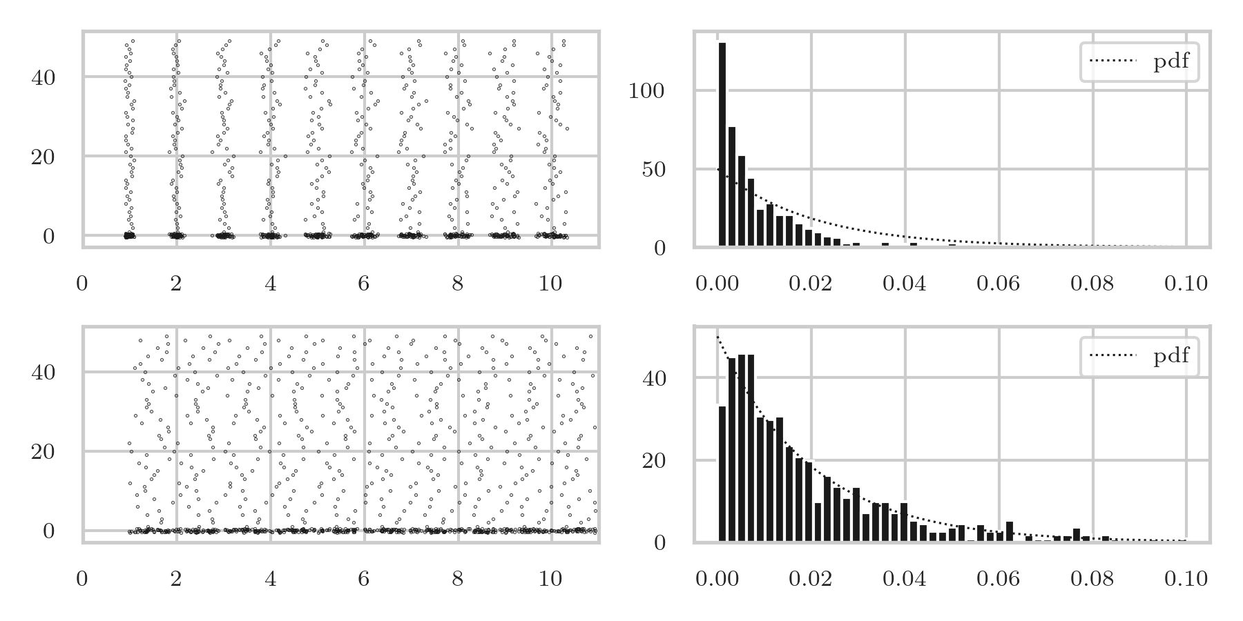
To conclude, the combined inter-arrival times in this simulation are approximately exponentially distributed. This approximation is useful in other systems fed by many mutually independent arrival streams, provided no single stream dominates.6You need strong arguments for other approximations. To avoid any confusion, here we model the inter-arrival times for one patient as uniformly distributed, but the same phenomenon occurs when the inter-arrival times for one patient have other types of distribution.
The arrival times above are sorted; Alg. 1.2.22 gives an algorithm for sorting a list.
It remains to formalize the observations from the above plots.7If you are not interested in probability theory, you can skip the rest of this section. In fact, we should distinguish between two limiting regimes. Patients recurrently plan appointments, separated around some mean period, that is, roughly every half a year. The upper left panel in Fig. 1.1 suggests that if the number of appointments increases, the appointments for each patient eventually become uniformly distributed on the period length (here half a year). The lower left panel suggests that if the appointments are uniformly distributed to begin with, they remain uniformly distributed. So, our first step is to prove that, as the number of visits increases, the arrival times modulo the cycle length become uniformly distributed over the cycle. The second claim is that, in the limit of many patients, each arriving at a uniformly distributed time in an interval, the inter-arrival times of all patients together become exponentially distributed, in a scaled sense.
The theorems and proofs are elegant and combine order statistics, the beta distribution, first-step analysis, and some infinitesimal calculus to give the reasoning a heuristic flavor. Finally, we discuss an important smoothing property of taking expectations. This idea is also relevant in data science when moving averages are used.
Let us first show that periodically planned arrivals, with some stochasticity, tend to become uniformly distributed over an interval. To formalize this claim, we consider a discrete-time model. There are on average \(C\) days between two successive visits of a patient (for the moment, the time on a day is of no importance). For instance, let the inter-arrival times \(X_{i}\) be such that \(\P{X_{i}=C-1} = \P{X_{i}=C+1}=1/2.\) In this case, if the process starts on day \(0\) and \(X_{1} = C-1,\) the next visit will be on day \(C-1,\) but if \(X_{1}=C+1,\) the next visit will be on day \(1\) of the next cycle. Looking at the arrival process like this, the patient moves on a circle with states \(\set{0, 1, \ldots, C-1},\) and with every visit the patient moves with probability \(1/2\) one state to the left or to the right. Thus, when \(X=C-1,\) we can just as well model this as \(X=-1.\)8There is a small subtlety when the cycle length is even and \(\P{X=C-1} = \P{X=C+1} = 1/2.\) As an even number is a multiple of \(2,\) the odd (even) days can only be visited after an odd (even) number of visits. The problem is easily resolved by assuming, in addition, that \(C\) is odd or \(\P{X = 0} > 0.\)
Theorem 1.4.1.
Assume that the arrival times \(\set{A_{i}}\) live on the circle space \(\set{0, 1, \ldots, C-1},\) i.e., \(A_{i} = (A_{i-1} + X_{i}) \bmod C.\) If \(\set{X_{k}}_{k=1}^{\infty}\) is a set of iid rvs such that \(\E{X_{k}} < \infty,\) \(\sup_{j}\P{X_{k} =j} < 1,\) and the greatest common divisor of \(C\) and all differences \(x-y\) between possible values of \(X_k\) is \(1,\) then \(\alpha_k(i) = \P{A_k=i},\) i.e., the probability that the \(k\)th arrival is on the \(i\)th day, converges to \(1/C\) as \(k\to\infty.\)
Proof
The condition \(\E{X_k}<\infty\) restricts attention to increments with a finite mean, although it is not needed for convergence on the finite circle. We need \(\sup_j\P{X_k=j}<1\) to exclude trivial rvs.9A rv \(X\) is trivial when \(\P{X=a} = 1\) for some \(a.\)
For the proof, assume for the moment that \(\P{X_{k} = 1}=p \in (0, 1)\) and \(\P{X_{k}=-1} = q=1-p,\) and let \(C\) be odd.8There is a small subtlety when the cycle length is even and \(\P{X=C-1} = \P{X=C+1} = 1/2.\) As an even number is a multiple of \(2,\) the odd (even) days can only be visited after an odd (even) number of visits. The problem is easily resolved by assuming, in addition, that \(C\) is odd or \(\P{X = 0} > 0.\) By first-step analysis,
\begin{equation*} \alpha_{k+1}(i) = p \alpha_k(i-1) + q \alpha_k(i+1). \end{equation*}Clearly, if \(\alpha_{k}(i)=1/C\) for all \(i,\) then \(\alpha_{k+1}(i) = 1/C\) also. However, if not all \(\alpha_{k}(\cdot)\) are equal, there must be at least one state \(i\) such that \(\alpha_k(i)\) is strictly larger than at least one of its neighbors, that is, \(\alpha_{k}(i) \geq \Max{\alpha_k(i-1), \alpha_k(i+1)}\) and \(\alpha_{k}(i) > \Min{\alpha_k(i-1),\alpha_k(i+1)}.\)10Observe that, for this argument, it is necessary that \(C\) is finite. But then, on the next visit,
\begin{equation*} \alpha_{k+1}(i) = p \alpha_k(i-1) + q \alpha_k(i+1) < \alpha_k(i). \end{equation*}In words, averaging smooths local peaks and troughs, although the global maximum need not decrease after every visit.
For general step distributions, the stated gcd condition ensures that, after sufficiently many visits, there is a positive probability of moving from any position to any other position.11If you are interested in maths: the positions form a finite irreducible and aperiodic Markov chain; hence some power of its transition matrix has only positive entries. Thus, after that many visits, every \(\alpha_k(i)\) is replaced by a weighted average of all the previous probabilities, with strictly positive weights. Unless all probabilities are equal, the maximum of these averages is strictly smaller than the previous maximum, and the minimum is strictly larger than the previous minimum. Let \(\epsilon>0\) be the smallest of these finitely many weights. Each such averaging step reduces the difference between the maximum and minimum to at most \(1-C\epsilon\) times its previous value. This difference therefore tends to zero. Since the probabilities sum to one, each \(\alpha_k(i)\) converges to \(1/C.\)
Clearly, the proof applies to any finite \(C=1, 2, \ldots.\) To see how to generalize the argument to the circle \([0, 1)\) on the reals, consider a continuous function \(f\) on the unit circle \(C.\) As the circle is compact and \(f\) continuous, \(f\) achieves its maximum \(f(\bar x)\) at \(\bar x,\) say. Suppose for some \(\epsilon>0\) there is set \(A_{\epsilon}(\bar x) = \set{x \in C: f(x) \leq f(\bar x) -\epsilon}\) such that \(\P{A_{\epsilon}(\bar x )} > 0.\) (If there is no such set for any \(\epsilon,\) then \(f\) is a constant.) But then \(\E{f(\bar x+X)} \leq (f(\bar x) -\epsilon) \P{A_{\epsilon}(\bar x)} + f(\bar x) (1-\P{A_{\epsilon}(\bar x)}) < f(\bar x).\) Again, taking an average over \(f\) makes the maximum smaller and the minimum larger.
Applied to the hospital, after many visits of a patient—each roughly half a year apart— the visits will appear to be uniformly distributed on a `circle’ of half-year length.
There is one point that remains about the lower left panel of Fig. 1.1; recall that for this panel we started the simulation with uniformly distributed arrival times. What is the distribution of the arrival times on the circle if we start like this? Let us analyze this for the case in which the inter-arrival times are uniform on \([0,1]\) and we take the circle as \(C=[0, 1).\) Observe that when \(C=[0, 1),\) \(U+V \bmod 1,\) that is, the sum of two iid uniform rvs on the circle, is just the fractional part of \(U + V.\)
Theorem 1.4.2.
Let \(Z=\sum_{i=1}^{n} U_{i}\) for \(n\) rvs \(U_{i}\iidsim \Unif{[0,1)}.\) The fractional part of \(Z,\) i.e., \(Z-\lfloor Z \rfloor,\) is uniformly distributed on \([0,1).\)12\(\lfloor x \rfloor\) is the integer part of \(x\in \R.\)
Proof
Realizing that the density of the sum of two uniform rvs on \([0,1]\) is a triangle with base \([0,2]\) and height \(1,\)
\begin{align*} \P{U +V- \lfloor{U+V} \rfloor \leq x} &= \P{U +V\leq x} + \P{1\leq U +V\leq 1 + x} \\ &= x^{2}/2 + (1/2 - (1-x)^{2} /2) = x. \end{align*}Therefore, the fractional part of the sum of two uniform rvs is uniform on \([0,1].\) We can apply this result successively through the summation in \(Z.\) More generally, if \(U\sim\Unif{[0,1)}\) and \(V\) is any independent rv, then \((U+V)\bmod1\) is uniform on \([0,1).\) Conditional on \(V=v,\) adding \(v\) simply rotates the uniform distribution around the circle. Thus, a uniform initial phase remains uniform when the inter-arrival times are distributed on \([0.9,1.1]\), as in our simulation.
We now deal with the case with many patients, that is, when the number \(n\) of patients goes to infinity. By the above results, we model the arrival times as rvs \(\set{U_k}_{k=1}^{n}\) such that \(U_{k}\iidsim \Unif{[0,1)}.\) Recall that in the simulation we sorted the arrival times of all patients together to obtain the ordered sequence of arrivals as seen by the hospital. In probabilistic terms, the hospital sees the order statistics of \(\set{U_k}_{k=1}^{n}.\) Write this as \(0=A^{n}_{0} <A^{n}_1 < A^n_2 < \cdots < A_n^{n}< A_{n+1}^{n} = 1.\)13We neglect the probability of simultaneous arrivals; these have probability zero. Define the size of the inter-arrivals as seen by the hospital as \(X_{k}^{n} = A_k^n - A_{k-1}^{n},\) \(k=1, \ldots, n+1.\)
As the population size \(n\) increases, the size of the first gap, i.e., the properly scaled arrival time of the first patient, becomes increasingly like an exponentially distributed random variable.14We need to scale with a factor \(n\) because the number of patients increases.
Lemma 1.4.3.
\begin{equation*} \lim_{n\to\infty} \P{A^n_1 \leq x/n} = \lim_{n\to\infty} \P{X^n_1 \leq x/n} =1- e^{-x},\quad x\geq0. \end{equation*}Proof
The probability that the smallest of \(n\) rvs is less than some \(x\) is the same as \(1\) minus the probability that all \(n\) rvs are larger than \(x.\) Therefore,
\begin{align*} \P{ A^n_1 \leq x/n} &= 1 - \P{\Min{U_{1}, \cdots, U_{n}} > x/n} = 1 - (1-x/n)^{n}, \end{align*}because \(\P{U_{i} > x/n} = 1-x/n,\) and the \(U_{i}\) are iid. The RHS converges to \(1-e^{-x}\) as \(n\to \infty.\) Finally, from the definition, \(X_1^n = A_1^n - A_0^{n} = A_1^{n}.\)
Next, we show that all the hospital inter-arrival times have the same density.
Lemma 1.4.4.
For \(r\in (0, 1),\) the density of the \(k\)th inter-arrival time is \(f_{X_{k}^n}(r) = n (1-r)^{n-1},\) for \(k=1, \ldots, n+1.\)
Proof
From the proof of the previous lemma we have \(\P{X_1^n \leq r} = 1- (1-r)^{n},\) therefore \(f_{X_{1}^{n}}(r) \d r = \P{X_1^n \in [r, r + \d r]} = n (1-r)^{n-1} \d r.\) By symmetry, \(X_1^n \sim X_{n+1}^{n}.\) It remains to deal with the intermediate inter-arrivals.
The probability of the event \(A_1^n < A_2^n < \cdots < A_{k-2}^n < x,\) \(A_{k-1}^n \in [x, x+ \d x], A_k^n \in [y, y+\d y],\) \(y < A_{k+1}^{n} < \cdots < A_n^{n}\) is given by
\begin{align*} f_{A_{k-1}^n, A_k^n}(x, y) \d x \d y = \frac{n!}{(k-2)!(n-k)!} x^{k-2} (1-y)^{n-k} \d x \d y, \end{align*}because \(k-2\) arrivals must occur before \(x,\) \(n-k\) after \(y\) and one arrival in \([x, x+\d x]\) and one in \([y, y+\d y].\) With this, the probability that \(X_k^{n} \in [r, r+\d r]\) becomes
\begin{align*} f_{X_{k}^n}(r) \d r = \d r \int_{0}^{1-r} f_{A_{k-1}^n, A_k^n}(x, x+r) \d x, \end{align*}because \(X_{k}^{n}= A_{k}^{n } -A_{k-1}^{n}= r \implies y = A_{k}^{n } = A_{k-1}^{n} + r = x +r,\) and \(x\) can lie anywhere in \([0, 1-r].\)
Substituting in this integral the density \(f_{A_{k-1}^n, A_k^n},\) but dropping the factorials for the moment for notational ease, we find
\begin{align*} \int_{0}^{1-r} x^{k-2} (1-r-x)^{n-k} \d x &= (1-r)^{n-2}\int_0^{1-r} \rb{\frac{x}{1-r}}^{k-2} \rb{ \frac{1-r - x}{1-r}}^{n-k} \d x\\ &= (1-r)^{n-1}\int_0^1 x^{k-2}(1-x)^{n-k} \d x \\ &= (1-r)^{n-1} \frac{(k-2)!(n-k)!}{(n-1)!}, \end{align*}where we use the normalization constant of the Beta distribution to compute the last integral. Canceling the factorials proves the claim.
Combining the above two lemmas leads straightaway to the next theorem.
Theorem 1.4.5.
Let \(n\) jobs arrive at a station such that the arrival times are rvs \(U_{k}\iidsim \Unif{[0,1]}.\) Then all inter-arrival times \(\set{X_{k}^{n}}_{k=1}^{n+1}\) as seen by the server (the hospital) have the same distribution. The common distribution of the scaled inter-arrival times \(nX_k^n\) converges to an exponential distribution with rate \(1\): \(\lim_{n\to\infty} \P{nX_{k}^{n}\leq x} = 1-e^{-x},\quad x\geq0.\)
Proof
By Lem. 1.4.4, the rvs \(\set{X_k^n}_{k=1}^{n}\) have the same density \(n(1-r)^{n-1}.\) By symmetry, \(X_{n+1}^n\) has this density too. By Lem. 1.4.3, \(\lim_{n\to\infty}\P{nX_k^n \leq x} = 1-e^{-x}\) for each \(k.\)