1.4 Probabilistic Arithmetic

In Section 1.2 we were interested in how the visiting times of a patient would become distributed over periods of half a year after many visits. We can formalize this problem as follows for one patient. Let \(X_k\) be the \(k\)th inter-arrival time, and write \(C\) for the length of the interval in which the patient has to see a doctor; here \(C\) is half a year. Then the times at which the arrivals are distributed over the periods behave like

To compute the distribution of \(Z_k\) we need to be able to compute the distribution of \(Y_{k} = Z_{k-1} + X_k\), and then find the distribution of \(f(Y_k)\) where \(f(x) = x \bmod C\). Clearly, this is a very unattractive task to carry out by hand. In this section we develop algorithms that allow a computer to carry out this tedious work.

More generally, later sections require numerical work to gain insight into the behavior of stochastic processes. We therefore develop a small collection of procedures for probabilistic arithmetic. The emphasis is on reusable algorithmic patterns: how probability distributions are stored, how procedures transform and combine random variables, and why these procedures work. At the end of this section, we use these algorithms to study the distribution of \(\{Z_k\}\) discussed above.

Let us start by making explicit what we mean by a pattern. As a first pattern, consider the \(+\) operator. Suppose that we only know how to do addition on the positive integers.¹¹For example: \(3+5=8\). Observe that the definition of addition on integers cannot be directly applied to rationals. To add fractions, we need to extend the symbol \(+\) to the following procedure: make the denominators of the fractions identical, and then add the numerators.²²\(1/3+1/2 = 2/6 + 3/6 = (2+3)/6 = 5/6\). However, this procedure does not work to compute \(\sqrt 2 + \sqrt 3\).³³\(\sqrt 2\) and \(\sqrt 3\) are not rationals so we cannot make the denominators equal. To add general real numbers, we need to extend the definition of \(+\) yet further.⁴⁴One way is like this: \(\sqrt 2 + \sqrt 3 = \sup\{x + y : x, y \in \Q, x^{2} \leq 2, y^{2} \leq 3\}\). Next, we need to define addition for complex numbers, vectors, matrices \ldots In summary, when learning mathematics, we have been silently \emph{overloading} the \(+\) operator to many different situations.

In our present case, we write \(X+Y\) for two independent rvs to mean the convolution:

where \(p_{i} = \P{X=i}\), \(q_j = \P{Y=j}\) and the indicator \(\1{A} = 1\) if the event \(A\) occurs, and \(0\) otherwise. Below we express this as an algorithm.⁵⁵For addition there exists a much faster method based on Fast Fourier transforms.

Thus, the first pattern that helps us to reason in more abstract ways about problems is to use operator overloading.

This brings us to a second pattern: observe that the expression \(X+Y\) combines two rvs \(X\) and \(Y\) and then applies some function. Similarly, the operations \(X-Y\), \(XY\), \(\max\{X, Y\}\) are all functions applied to two independent rvs. What we therefore need is a method to compute the pmf of a new rv \(f(X,Y)\), where \(f\) is some general \emph{binary} function.⁶⁶A binary function depends on two arguments.

We identify a third pattern when we realize that to compute \(\V X\), we need \(\E{X^{2}}\). But \(\E{X^{2}}\) is the expectation of the rv \(g(X)\) where \(g(x) = x^{2}\). So, we also need a method to compute the pmf of the rv \(g(X)\), where now \(g\) is some general \emph{unary} function.⁷⁷A unary function depends on just one argument.

In summary, we want to develop procedures that support the following operations on rvs:

1. operator overloading for addition, subtraction, and potentially other arithmetical operations,
2. the application of a unary function to obtain a new rv
3. the application of a binary function.

We call these procedures probabilistic arithmetic, and we will develop, step by step, clear and general algorithms to support this. However, we first need to introduce some computer science concepts.

A useful data structure for storing the pmf of a discrete rv is a map. Its keys are the possible values of the rv, and the value stored under each key is its probability. Since values outside the support have probability zero, we use the default value zero. We denote the pmf map of an rv \(X\) by \(p_X\), so that \(p_X(x)=\P{X=x}\).

\begin{algorithm}
\caption{Store two probability mass functions.}
\begin{algorithmic}[1]
\State \textbf{Input:} none
\State \textbf{Output:} pmf maps \(p_X,p_Y\)
\State \(p_X\gets\pr{Map}()\)
\State \(p_X(1)\gets1/2\), \(p_X(2)\gets1/2\)
\State \(p_Y\gets\pr{Map}()\)
\State \(p_Y(1)\gets1/2\), \(p_Y(2)\gets1/2\)
\end{algorithmic}

\end{algorithm}

It is obvious that the pmf map \(p_Z\) for \(Z=X+Y\) should satisfy \(p_Z(2)=1/4\), \(p_Z(3)=1/2\), and \(p_Z(4)=1/4\). Let us use (1.4.1) to compute the pmf of \(Z=X+Y\).

\begin{algorithm}
\caption{Compute the pmf of the sum.}
\begin{algorithmic}[1]
\State \textbf{Input:} pmf maps \(p_X,p_Y\)
\State \textbf{Output:} pmf map \(p_Z\) for \(X+Y\)
\State \(p_Z\gets\pr{Map}()\)
\For{\(i\in\qb{1,2}\)}
    \For{\(j\in\qb{1,2}\)}
        \State \(p_Z(i+j)\gets p_Z(i+j)+p_X(i)p_Y(j)\)
    \EndFor
\EndFor
\Return \(p_Z\)
\end{algorithmic}

\end{algorithm}

Because \(p_Z\) is a map with default value zero, the first contribution to a key is added to zero. Later contributions are added to the value already stored under that key. In particular, the two pairs \((1,2)\) and \((2,1)\) each add \(1/4\) to \(p_Z(3)\). Thus, the algorithm returns \(p_Z(2)=1/4\), \(p_Z(3)=1/2\), and \(p_Z(4)=1/4\).

\newthought{The above algorithm} assumes that mathematically equal keys have the same representation in the computer. This requires care when the keys are stored as floating-point numbers. Most real numbers cannot be represented exactly with finitely many digits. Consequently, two expressions that are mathematically equal, such as \(1/3\) and \(1-2/3\), can be stored as slightly different numbers. An implementation of \pr{Map} in a real computer language then treats them as different keys and does not combine their probabilities. This is a general problem of computer arithmetic, not a problem specific to a programming language. We avoid it by using exact numbers, such as integers or fractions, whenever possible. Otherwise, we round all keys to an agreed precision before storing them.

The procedure \(\pr{ToFraction}\) of Alg. 1.4.3 replaces a number \(x\in \R\) by a nearby fraction, rounded to \(d\) decimal places. It first uses denominator \(10^d\) and then reduces the fraction using the greatest common divisor.⁸⁸The greatest common divisor can be computed with Euclid’s algorithm. See Euclidean algorithm for its implementation. Keeping this conversion in a separate procedure hides its details from the algorithms that use it. If we later change the precision or the conversion rule, we only have to change \(\pr{ToFraction}\).

\begin{algorithm}
\caption{Convert a number to a fraction.}
\begin{algorithmic}[1]
\State \textbf{Input:} a number \(x\) and precision \(d\)
\State \textbf{Output:} a reduced fraction \(a/b\)
\Procedure{ToFraction}{\(x,d = 10\)}
    \State \(q\gets10^d\)
    \State \(p\gets\operatorname{round}(xq)\)
    \State \(g\gets\pr{GCD}(|p|,q)\)
    \State \(a\gets p/g\), \(b\gets q/g\)
    \Return \(a/b\)
\EndProcedure
\end{algorithmic}

\end{algorithm}

The procedure \(\pr{MakePMF}\) of Alg. 1.4.4 uses the conversion to fractions to construct a pmf map from a map of outcomes and non-negative weights. It first converts every outcome with \(\pr{ToFraction}\). When two outcomes are converted to the same fraction, their weights are added. Finally, \(\pr{NormalizeMap}\), Alg. 1.4.5, makes the stored weights sum to one.

\begin{algorithm}
\caption{Construct a probability mass function.}
\begin{algorithmic}[1]
\State \textbf{Input:} a finite map \(w\) with non-negative values and positive sum
\State \textbf{Output:} a pmf map \(p\)
\Procedure{MakePMF}{\(w\)}
    \State \(r\gets\pr{Map}()\)
    \For{\(x\in\pr{Keys}(w)\)}
        \State \(y\gets\pr{ToFraction}(x)\)
        \State \(r(y)\gets r(y)+w(x)\)
    \EndFor
    \Return \(\pr{NormalizeMap}(r)\)
\EndProcedure
\end{algorithmic}

\end{algorithm}

The procedure \(\pr{Normalize}\) of Alg. 1.1.10 normalizes a list of weights. For a pmf, we store the weights in a map whose keys are the possible outcomes. The procedure \(\pr{NormalizeMap}\) of Alg. 1.4.5 carries out the same calculation while preserving these keys. It first removes entries whose relative weight does not exceed the numerical threshold \(\epsilon=10^{-16}\), and then normalizes the remaining weights.

\begin{algorithm}
\caption{Normalize the values stored in a map.}
\begin{algorithmic}[1]
\State \textbf{Input:} a finite map \(w\) with non-negative values and positive sum; threshold \(\epsilon\)
\State \textbf{Output:} a map \(p\) whose values sum to one
\Procedure{NormalizeMap}{\(w,\epsilon = 10^{-16}\)}
    \State \(T\gets\pr{Sum}\rb{\pr{Values}(w)}\)
    \State \(S\gets\qb{q:q\in\pr{Keys}(w),\ w(q)/T>\epsilon}\)
    \State \(\var{total}\gets\pr{Sum}\rb{\qb{w(q):q\in S}}\)
    \State \(p\gets\pr{Map}()\)
    \For{\(q\in S\)}
        \State \(p(q)\gets w(q)/\var{total}\)
    \EndFor
    \Return \(p\)
\EndProcedure
\end{algorithmic}

\end{algorithm}

As a last abstraction we introduce so-called \(\lambda\) function. Sometimes functions are so short and simple that we simply do not want to bother to give them a name. For such cases, the \(\lambda\) function serves as an anonymous function. We write \(\lambdafun{x}{h(x)}\) for the function that takes \(x\) as its argument and returns \(h(x)\). Let’s see how to use this concept to compute the different moments of a rv \(X\).

The procedure \(\pr{Expectation}\) applies \(f\) to every possible value of the rv represented by \(p_X\) to compute \(\E{f(X)}\). With this, Alg. 1.4.7 computes the mean and variance with calls to simple \(\lambda\) functions.

\begin{algorithm}
\caption{Compute the expectation of functions of a discrete random variable \(X\).}
\begin{algorithmic}[1]
\State \textbf{Input:} pmf map \(p_X\), function \(f\)
\State \textbf{Output:} \(\E{f(X)}\)
\Procedure{Expectation}{\(p_X,f\)}
    \State \(\var{terms}\gets\qb{f(x)p_X(x):x\in\pr{Keys}(p_X)}\)
    \Return \(\pr{Sum}\rb{\var{terms}}\)
\EndProcedure
\end{algorithmic}

\end{algorithm}

\begin{algorithm}
\caption{Compute moments of a discrete random variable.}
\begin{algorithmic}[1]
\State \textbf{Input:} pmf map \(p_X\)
\State \textbf{Output:} mean, second moment, variance, and standard deviation of \(X\)
\Procedure{Mean}{\(p_X\)}
    \Return \(\pr{Expectation}(p_X,\lambdafun{x}{x})\)
\EndProcedure
\Procedure{SecondMoment}{\(p_X\)}
    \Return \(\pr{Expectation}(p_X,\lambdafun{x}{x^2})\)
\EndProcedure
\Procedure{Variance}{\(p_X\)}
    \Return \(\pr{SecondMoment}(p_X)-\pr{Mean}(p_X)^2\)
\EndProcedure
\Procedure{StandardDeviation}{\(p_X\)}
    \Return \(\sqrt{\pr{Variance}(p_X)}\)
\EndProcedure
\end{algorithmic}

\end{algorithm}

Another nice example is the cdf, since \(\P{X\leq x}=\E{\1{X\leq x}}\).

\begin{algorithm}
\caption{Compute the cdf through expectation.}
\begin{algorithmic}[1]
\State \textbf{Input:} pmf map \(p_X\), value \(x\)
\State \textbf{Output:} cdf value \(F_X(x)\)
\Procedure{CDF\_slow}{\(p_X,x\)}
    \Return \(\pr{Expectation}(p_X,\lambdafun{y}{\1{y \leq x}})\)
\EndProcedure
\end{algorithmic}

\end{algorithm}

Computing the CDF works faster with search sorted. We discuss here how to set this up.

First, sort the support of \(X\):

The probabilities in this same order form the list

Applying \(\pr{CumSum}\) to \(P\) gives

The procedure \(\pr{CumSum}\) constructs the cumulative sums. Its \(k\)th output is the sum of the first \(k\) inputs. For example, \(\pr{CumSum}(\qb{2,3,1})=\qb{2,5,6}\).

\begin{algorithm}
\caption{Compute the cumulative sums of a list.}
\begin{algorithmic}[1]
\State \textbf{Input:} a list \(A=\qb{a_1,\ldots,a_n}\)
\State \textbf{Output:} a list \(C=\qb{c_1,\ldots,c_n}\), where \(c_k=\sum_{i=1}^k a_i\)
\Procedure{CumSum}{\(A\)}
    \State \(C\gets\qb{}\), \(\var{total}\gets0\)
    \For{\(k=1,\ldots,n\)}
        \State \(\var{total}\gets\var{total}+a_k\)
        \State \(c_k\gets\var{total}\)
    \EndFor
    \Return \(C\)
\EndProcedure
\end{algorithmic}

\end{algorithm}

\(\pr{PrepareCDF}\) stores the cumulative sum \(c_k\) under key \(s_k\) in the map \(F_X\). Hence

\begin{algorithm}
\caption{Prepare the support and cumulative probabilities of a discrete random variable.}
\begin{algorithmic}[1]
\State \textbf{Input:} pmf map \(p_X\)
\State \textbf{Output:} cumulative-probability map \(F_X\)
\Procedure{PrepareCDF}{\(p_X\)}
    \State \(S\gets\pr{Sort}(\pr{Keys}(p_X))\)
    \State \(C\gets\pr{CumSum}(\qb{p_X(s_1),\ldots,p_X(s_n)})\)
    \State \(F_X\gets\pr{Map}()\)
    \For{\(k=1,\ldots,n\)}
        \State \(F_X(s_k)\gets c_k\)
    \EndFor
    \Return \(F_X\)
\EndProcedure
\end{algorithmic}

\end{algorithm}

To find the cdf \(\P{X\leq x}\) from the prepared map \(F_X\), it now suffices to find how many of its keys are no larger than \(x\). \(\pr{SearchSorted}\) offers this functionality.⁹⁹Like sorting, efficiently searching sorted data is used almost everywhere that computers are used. The ideas behind are this algorithm are very important. It inspects the middle of the current part of the list and then calls itself on either the left or the right part. Each call therefore reduces the part that remains to be searched by about one half, so only about¹⁰¹⁰\(\log\) is the natural logarithm, \(\log_2\) has base 2. \(\log_2 n\) comparisons are needed for a list of length \(n\).

\begin{algorithm}
\caption{Find how many entries of a sorted list are  \(\leq x\).}
\begin{algorithmic}[1]
\State \textbf{Input:} a sorted list \(A=\qb{a_1,\ldots,a_n}\) and a number \(x\)
\State \textbf{Output:} the number of entries in \(A\) that are at most \(x\)
\Procedure{SearchSorted}{\(A,x,l=1,r=n\)}
    \If{\(l>r\)}
        \Return \(r\)
    \EndIf
    \State \(m\gets\lfloor(l+r)/2\rfloor\)
    \If{\(a_m\leq x\)}
        \Return \(\pr{SearchSorted}(A,x,m+1,r)\)
    \EndIf
    \Return \(\pr{SearchSorted}(A,x,l,m-1)\)
\EndProcedure
\end{algorithmic}

\end{algorithm}

The returned value is zero when \(x<s_1\). Otherwise it is the largest index \(k\) for which \(s_k\leq x\), and the cdf is simply \(F_X(s_k)\).

The procedure \(\pr{CDF}\) first prepares the internal cdf map \(F_X\). It then returns an inner function \(F\). This function retains access to \(F_X\). Its keys are the support in increasing order because \(\pr{PrepareCDF}\) inserted them in that order. Each call to \(F\) therefore only has to run \(\pr{SearchSorted}\) on these keys and retrieve the corresponding value from \(F_X\).

\begin{algorithm}
\caption{Construct a cdf that uses search sorted.}
\begin{algorithmic}[1]
\State \textbf{Input:} pmf map \(p_X\)
\State \textbf{Output:} cdf procedure \(F\)
\Procedure{CDF}{\(p_X\)}
    \State \(F_X\gets\pr{PrepareCDF}(p_X)\)
    \State \(S\gets\pr{Sort}(\pr{Keys}(F_X))\) \Comment{\(S=\qb{s_1,\ldots,s_n}\)}
    \Procedure{F}{\(x\)}
        \State \(k\gets\pr{SearchSorted}(S,x)\)
        \If{\(k=0\)}
            \Return \(0\)
        \EndIf
        \Return \(F_X(s_k)\)
    \EndProcedure
    \Return \(F\)
\EndProcedure
\end{algorithmic}

\end{algorithm}

For \(F\gets\pr{CDF}(p_X)\), the survivor function follows immediately, since \(\P{X>x}=1-\P{X\leq x}=1-F(x)\).

\begin{algorithm}
\caption{Compute the survivor function from the cdf.}
\begin{algorithmic}[1]
\State \textbf{Input:} cdf \(F\), value \(x\)
\State \textbf{Output:} survivor probability \(1-F(x)\)
\Procedure{Survivor}{\(F,x\)}
    \Return \(1-F(x)\)
\EndProcedure
\end{algorithmic}

\end{algorithm}

We can now also generate simulated realizations of \(X\). Let \(U\sim\Unif{[0,1]}\). The inverse-cdf method returns the smallest support value \(s_k\) for which \(F_X(s_k)\geq U\). This has the required distribution because

The procedure \(\pr{Simulate}\) applies \(\pr{SearchSorted}\) to the cumulative probabilities. When \(U=c_k\), it returns \(s_k\); otherwise it returns the next support value \(s_{k+1}\). The special case \(k=0\) returns the first support value.

\begin{algorithm}
\caption{Generate \(N\) simulated realizations of a discrete random variable.}
\begin{algorithmic}[1]
\State \textbf{Input:} pmf map \(p_X\), number of draws \(N\)
\State \textbf{Output:} \(N\) simulated values
\Procedure{Simulate}{\(p_X,N=1\)}
    \State \(F_X\gets\pr{PrepareCDF}(p_X)\)
    \State \(S\gets\pr{Sort}(\pr{Keys}(F_X))\)
    \State \(C\gets\qb{F_X(s_1),\ldots,F_X(s_n)}\)
    \For{\(j=1,\ldots,N\)}
        \State Generate \(u\sim\Unif{[0,1]}\)
        \State \(k\gets\pr{SearchSorted}(C,u)\)
        \If{\(k=0\)}
            \State \(r_j\gets s_1\)
        \ElsIf{\(c_k=u\)}
            \State \(r_j\gets s_k\)
        \Else
            \State \(r_j\gets s_{k+1}\)
        \EndIf
    \EndFor
    \Return \(\qb{r_1,\ldots,r_N}\)
\EndProcedure
\end{algorithmic}

\end{algorithm}

The two remaining patterns are binary and unary functions. Supporting binary functions works the same as addition in (1.4.1). The procedure \(\pr{BinaryTransform}\) replaces the particular function \(x+y\) by a general binary function \(f(x,y)\). When several pairs produce the same value \(z\), their probability masses accumulate in the pmf map \(p_Z\).

\begin{algorithm}
\caption{Construct the pmf of \(f(X,Y)\) where \(X,Y\) are independent rvs.}
\begin{algorithmic}[1]
\State \textbf{Input:} pmf maps \(p_X,p_Y\) of independent rvs, binary function \(f\)
\State \textbf{Output:} pmf map of \(f(X,Y)\)
\Procedure{BinaryTransform}{\(p_X,p_Y,f\)}
    \State \(p_Z\gets\pr{Map}()\)
    \For{\(x\in\pr{Keys}(p_X)\)}
        \For{\(y\in\pr{Keys}(p_Y)\)}
            \State \(z\gets f(x,y)\)
            \State \(p_Z(z)\gets p_Z(z)+p_X(x)p_Y(y)\)
        \EndFor
    \EndFor
    \Return \(\pr{MakePMF}(p_Z)\)
\EndProcedure
\end{algorithmic}

\end{algorithm}

For a unary function \(f\), let \(Z=f(X)\). Its pmf satisfies

The procedure \(\pr{UnaryTransform}\) implements this rule by applying \(f\) to each possible value of \(X\). Different values of \(X\) can produce the same value \(z=f(x)\), so their probability masses accumulate in the pmf map \(p_Z\).

\begin{algorithm}
\caption{Construct the pmf of \(f(X)\).}
\begin{algorithmic}[1]
\State \textbf{Input:} pmf map \(p_X\), function \(f\)
\State \textbf{Output:} pmf map of \(f(X)\)
\Procedure{UnaryTransform}{\(p_X,f\)}
    \State \(p_Z\gets\pr{Map}()\)
    \For{\(x\in\pr{Keys}(p_X)\)}
        \State \(z\gets f(x)\)
        \State \(p_Z(z)\gets p_Z(z)+p_X(x)\)
    \EndFor
    \Return \(\pr{MakePMF}(p_Z)\)
\EndProcedure
\end{algorithmic}

\end{algorithm}

With these two transform procedures, we can now define many useful functions of rvs.

A constant rv takes one value (c) with probability one. Its pmf is useful as the starting point for several of the procedures below.

\begin{algorithm}
\caption{Construct the pmf of a constant rv.}
\begin{algorithmic}[1]
\State \textbf{Input:} value \(c\)
\State \textbf{Output:} pmf map concentrated at \(c\)
\Procedure{Constant}{\(c\)}
    \State \(p_c\gets\pr{Map}()\), \(p_c(c)\gets1\)
    \Return \(p_c\)
\EndProcedure
\end{algorithmic}

\end{algorithm}

Addition is the special case of \(\pr{BinaryTransform}\) obtained by taking \(f(x,y)=x+y\).

\begin{algorithm}
\caption{Add two independent rvs.}
\begin{algorithmic}[1]
\State \textbf{Input:} pmf maps \(p_X,p_Y\) of independent rvs
\State \textbf{Output:} pmf map of \(X+Y\)
\Procedure{Add}{\(p_X,p_Y\)}
    \Return \(\pr{BinaryTransform}\rb{p_X,p_Y,\lambdafun{(x,y)}{x+y}}\)
\EndProcedure
\end{algorithmic}

\end{algorithm}

The \(N\)-fold convolution of \(p_X\) is the pmf of \(X_1+\cdots+X_N\), where the \(X_k\) are independent copies of \(X\). For \(N=0\), the sum is zero.

\begin{algorithm}
\caption{Construct the pmf of the sum of \(N\) independent copies of an rv.}
\begin{algorithmic}[1]
\State \textbf{Input:} pmf map \(p_X\), number of copies \(N\)
\State \textbf{Output:} pmf map of the sum of \(N\) independent copies of \(X\)
\Procedure{Convolution}{\(p_X,N\)}
    \State \(p_Z\gets\pr{Constant}\rb{0}\)
    \For{\(k=1,\ldots,N\)}
        \State \(p_Z\gets\pr{Add}\rb{p_Z,p_X}\)
    \EndFor
    \Return \(p_Z\)
\EndProcedure
\end{algorithmic}

\end{algorithm}

The unary transform allows us to define \(-X\) as an rv: unary minus reflects all outcomes about zero.

\begin{algorithm}
\caption{Negate an rv.}
\begin{algorithmic}[1]
\State \textbf{Input:} pmf map \(p_X\)
\State \textbf{Output:} pmf map of \(-X\)
\Procedure{Negate}{\(p_X\)}
    \Return \(\pr{UnaryTransform}\rb{p_X,\lambdafun{x}{-x}}\)
\EndProcedure
\end{algorithmic}

\end{algorithm}

We can now implement subtraction as addition of the negative.

\begin{algorithm}
\caption{Subtract two independent rvs.}
\begin{algorithmic}[1]
\State \textbf{Input:} pmf maps \(p_X,p_Y\) of independent rvs
\State \textbf{Output:} pmf map of \(X-Y\)
\Procedure{Subtract}{\(p_X,p_Y\)}
    \Return \(\pr{Add}\rb{p_X,\pr{Negate}\rb{p_Y}}\)
\EndProcedure
\end{algorithmic}

\end{algorithm}

The minimum of two independent rvs is another useful binary transform.

\begin{algorithm}
\caption{Take the minimum of two independent rvs.}
\begin{algorithmic}[1]
\State \textbf{Input:} pmf maps \(p_X,p_Y\) of independent rvs
\State \textbf{Output:} pmf map of \(\min\{X,Y\}\)
\Procedure{Minimum}{\(p_X,p_Y\)}
    \Return \(\pr{BinaryTransform}\rb{p_X,p_Y,\lambdafun{(x,y)}{\min\{x,y\}}}\)
\EndProcedure
\end{algorithmic}

\end{algorithm}

Likewise, we define the maximum of two independent rvs.

\begin{algorithm}
\caption{Take the maximum of two independent rvs.}
\begin{algorithmic}[1]
\State \textbf{Input:} pmf maps \(p_X,p_Y\) of independent rvs
\State \textbf{Output:} pmf map of \(\max\{X,Y\}\)
\Procedure{Maximum}{\(p_X,p_Y\)}
    \Return \(\pr{BinaryTransform}\rb{p_X,p_Y,\lambdafun{(x,y)}{\max\{x,y\}}}\)
\EndProcedure
\end{algorithmic}

\end{algorithm}

The positive part satisfies \(X^+=\max\{0,X\}\). We therefore construct a constant rv equal to zero and take its maximum with \(X\).

\begin{algorithm}
\caption{Take the positive part of an rv.}
\begin{algorithmic}[1]
\State \textbf{Input:} pmf map \(p_X\)
\State \textbf{Output:} pmf map of \(X^+\)
\Procedure{PositivePart}{\(p_X\)}
    \Return \(\pr{Maximum}\rb{\pr{Constant}\rb{0},p_X}\)
\EndProcedure
\end{algorithmic}

\end{algorithm}

Likewise, \(X^-=\max\{0,-X\}=[-X]^+\), so we first negate \(X\) and then take its positive part.

\begin{algorithm}
\caption{Take the negative part of an rv.}
\begin{algorithmic}[1]
\State \textbf{Input:} pmf map \(p_X\)
\State \textbf{Output:} pmf map of \(X^-\)
\Procedure{NegativePart}{\(p_X\)}
    \Return \(\pr{PositivePart}\rb{\pr{Negate}\rb{p_X}}\)
\EndProcedure
\end{algorithmic}

\end{algorithm}

Taking outcomes modulo \(C\) is also a unary transform.

\begin{algorithm}
\caption{Reduce the outcomes of an rv modulo \(C\).}
\begin{algorithmic}[1]
\State \textbf{Input:} pmf map \(p_X\), modulus \(C\)
\State \textbf{Output:} pmf map of \(X\bmod C\)
\Procedure{Modulo}{\(p_X,C\)}
    \Return \(\pr{UnaryTransform}\rb{p_X,\lambdafun{x}{x\bmod C}}\)
\EndProcedure
\end{algorithmic}

\end{algorithm}

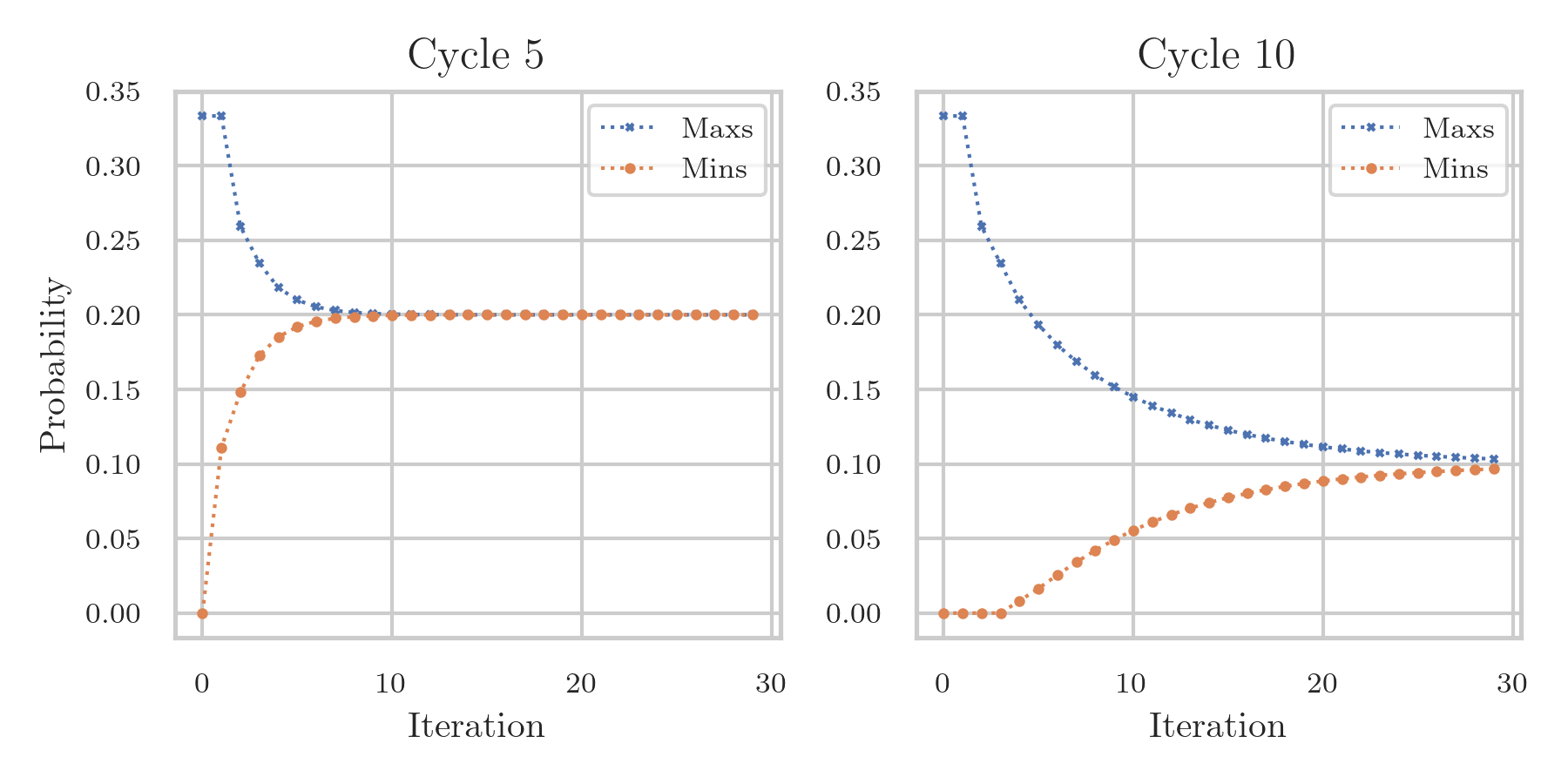
With these procedures we can study the content of Th. 1.3.1 numerically. In particular, how quickly do the arrival times on the circle converge to the uniform distribution? Recall that

We first use \(\pr{Add}\), and then use \(\pr{Modulo}\).

In Alg. 1.4.27 we iteratively compute the arrival-time position \(\sum_{i=1}^{n}X_i\bmod C\), where \(X_i\sim\Unif{\{-1,0,1\}}\) and \(A_0=0\). We track the positions that occur with the smallest and largest probability. Fig. 1.1 shows the result.

\begin{algorithm}
\caption{Track convergence of the arrival-time distribution on a cycle.}
\begin{algorithmic}[1]
\State \textbf{Input:} cycle length \(C\), number of iterations \(n\), and step pmf \(p_X\)
\State \textbf{Output:} smallest and largest probabilities \(m_k,M_k\)
\Procedure{ArrivalConvergence}{\(C,n,p_X\)}
    \State \(p_{A_0}\gets\pr{Constant}\rb{0}\)
    \For{\(k=1,\ldots,n\)}
        \State \(p_{A_k}\gets\pr{Modulo}\rb{\pr{Add}\rb{p_{A_{k-1}},p_X},C}\)
        \State \(m_k\gets\min\qb{p_{A_k}(a):a=0,\ldots,C-1}\)
        \State \(M_k\gets\max\qb{p_{A_k}(a):a=0,\ldots,C-1}\)
    \EndFor
    \Return \(\qb{m_1,\ldots,m_n},\qb{M_1,\ldots,M_n}\)
\EndProcedure
\end{algorithmic}

\end{algorithm}

\begin{algorithm}
\begin{algorithmic}[1]
\State \(p_Z\gets\pr{Map}()\)
\For{\(x\in\pr{Keys}(p_X)\)}
    \For{\(y\in\pr{Keys}(p_Y)\)}
        \State \(z\gets f(x,y)\)
        \State \(p_Z(z)\gets p_Z(z)+\text{???}\)
    \EndFor
\EndFor
\end{algorithmic}

\end{algorithm}

\begin{algorithm}
\begin{algorithmic}[1]
\Procedure{SearchSorted}{\(A,x,l=1,r=n\)}
    \If{\(l>r\)}
        \Return \(r\)
    \EndIf
    \State \(m\gets\lfloor(l+r)/2\rfloor\)
    \If{\(a_m\leq x\)}
        \Return \(\pr{SearchSorted}(A,x,\text{???},r)\)
    \EndIf
    \Return \(\pr{SearchSorted}(A,x,l,m-1)\)
\EndProcedure
\end{algorithmic}

\end{algorithm}