
2.3 General Behavior of Queueing Systems
2.3 General Behavior of Queueing Systems
In this section, we develop a simulation environment for queueing systems to explore their behavior and visualize queue-length dynamics.
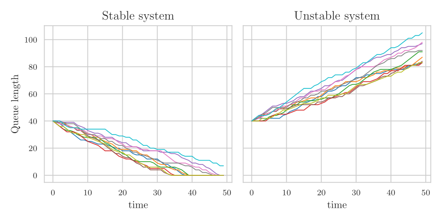
The first aspect to address is system stability. Intuitively, when work arrives faster than it can be served, on average, the queue grows; if work arrives slower, the queue remains close to the origin. To illustrate this, Fig. 2.1 shows queue-length sample paths for several arrival rates and service capacities.
import numpy as np
import matplotlib.pyplot as plt
import seaborn as sns

sns.set_style("whitegrid")
tex_fonts = {
    "text.usetex": True,
    "font.family": "fourier",
    "axes.labelsize": 10,
    "font.size": 10,
    "legend.fontsize": 8,
    "xtick.labelsize": 8,
    "ytick.labelsize": 8,
}

plt.rcParams.update(tex_fonts)
Let \(a_k\) be the number of arrivals and \(c_k\) the service capacity in period \(k\). We write
\begin{align*} \lambda &= \E{a_k}, & \mu &= \E{c_k}. \end{align*}We use Alg. 2.2.1 to compute the sample paths; jobs arriving in period \(k\) can be served in that same period. We simulate \(n=50\) periods with initial queue length \(L_0=40\) and mean arrival rate \(\lambda=6\). For each of ten independent sample paths, the arrivals \(a_k\) are uniformly distributed on \(\{5,6,7\}\), while the service capacity is constant at \(c_k=7\), and hence \(\mu=7\). The resulting stable queue-length trajectories are shown in the left panel of Fig. 2.1. For the right panel, we repeat the experiment with constant service capacity \(c_k=5\), and hence \(\mu=5\). Since \(\mu<\lambda\), the queue has positive drift and is unstable.
How about reducing the difference between \(\lambda\) and \(\mu\)? When \(\mu\) barely exceeds \(\lambda\), large fluctuations take longer to die out. To see this in quantitative terms, we run two simulations with smaller values for \(\mu\) while keeping \(\lambda=6\), and we compute the mean and variance of the number of jobs in the system.
For the first experiment, let \(c_k=6+B_k\), where \(B_k\sim\Bern{1/2}\) independently. Then \(\E{c_k}=6.5\). With \(n=5000\), \(L_0=0\), and the same arrival distribution as above, the simulation gives a sample mean queue length of \(0.45\) and a sample variance of \(0.64\).
For the second experiment, let \(c_k=6+B_k\), where \(B_k\sim\Bern{1/10}\) independently, so \(\mu=\E{c_k}=6.1\). With the same run length, initial queue length, and arrival distribution as above, the sample mean queue length is \(4.36\) and the sample variance is \(25.30\). Thus, reducing the excess service capacity from \(0.5\) to \(0.1\) substantially increases both the mean and the variance of the queue length.
Would variability affect the average queue length? We may suspect this because when \(a_{k}=1\) and \(c_{k}=1\) for all \(k\) and \(L_{0} = 0\), \(L_{k} = 0\) for all \(k\). If instead \(c_{i}=5\) when \(i\) is a multiple of \(5\) and \(0\) otherwise, queues do appear and disappear.1Observe that the mean service time is still 1; only the periods in which service is offered changed. Let us use simulation to see how variability can influence the queue-length process. The goal is now to make Fig. 2.2.
We first need a way to quantify relative variability. Suppose the standard deviation of the service time is \(1\) minute. If the mean service time is 1 hour, we are inclined to call the service times very regular, while if the mean is just 1 minute, we would call it irregular. To capture this relative effect, we define the square coefficient of variation (scv) of the rv \(X\) as2The scv is unit-less.
\begin{equation*} C^2_{X}:= \frac{\V X}{(\E X)^2}. \end{equation*}Continuing with the simulation, we seek a probability distribution for \(\{c_{k}\}\) with mean \(\mu\) and scv \(c^{2}\). A simple way to achieve this is to use a rv \(X\) such that \(\P{X=b} = p\) and \(\P{X=0} = 1-p\), and require that \(\E X = p b = \mu\) and \(C^2_X = c^{2}\). Using \(\V X = \E{X^{2}} - (\E X)^{2}\), we see that \(C^{2}_{X} = \E{X^{2}}/(\E X)^{2} - 1\). Rewriting, we get \(\E{X^{2}} = \mu^{2}(c^2+1)\), but we also know that \(\E{X^{2}} = p b^{2}\) for a Bernoulli-distributed rv. Solving for \(b\) and \(p\) in terms of \(\mu\) and \(c^{2}\) gives \(p = 1 / (1 + c^{2})\) and \(b=\mu/p = \mu (1+c^{2})\).
Thus, independent copies of \(X=bB\), with \(B\sim\Bern{p}\), provide a sequence with mean \(\mu\) and the required scv.
We simulate \(n=5000\) periods with \(L_0=0\), \(\lambda=6\), and \(\mu=6.5\), and compare scv values \(0.5\), \(1\), and \(2\). In the left panel of Fig. 2.2, arrivals are constant, \(a_k=6\), while the service capacities follow the two-point distributions constructed above. In the right panel, both arrivals and service capacities follow such distributions with the same scv. Applying the queue-length algorithm in each case shows that greater relative variability produces larger queue-length fluctuations.
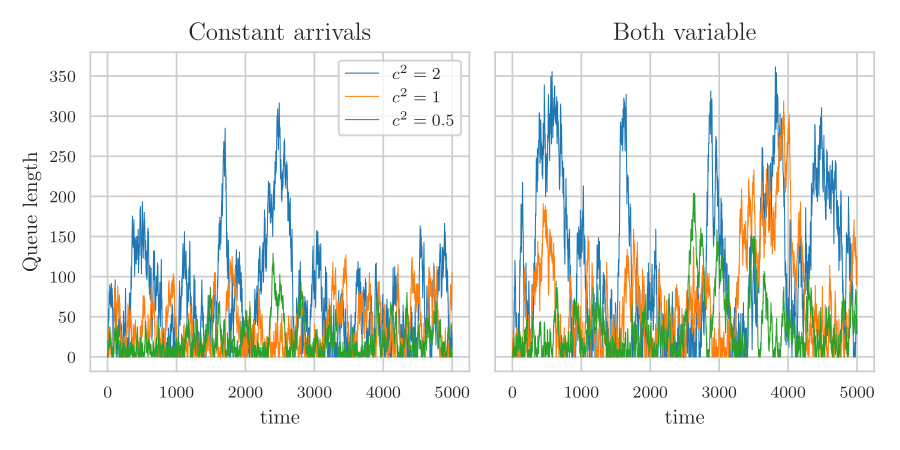
In conclusion, tight capacity or high relative variability leads to large queues. To improve performance, we have basically four options: increase capacity, reduce load (or demand), reduce the scv of the arrivals or of the services.3Of course, these options are not exclusive; for example, we can try to reduce the variability of the service process and add some capacity at the same time.
2.3.1 Proposal 9: Introduce tandem queues directly
Finally, we consider queues in sequence. For example, obtaining grades for a course involves several sequential steps. First, I grade the exams (and handle all changes that might occur during the review). I send a csv file with the grades to the secretary who uploads it. The secretary prints the file for me to sign, after which it is logged by the administration. In abstract terms, there are three stations (me, the secretary, and the back office), and I am involved at least twice, once for the grading and a second time for the signing. More generally, most service systems involve multiple servers visited4Perhaps even multiple times. to complete a service.
Finally, we consider queues in sequence.5For example, obtaining grades for a course involves several sequential steps. First, I grade the exams (and handle all changes that might occur during the review). I send a csv file with the grades to the secretary who uploads it. The secretary prints the file for me to sign, after which it is logged by the administration. In abstract terms, there are three stations (me, the secretary, and the back office), and I am involved at least twice, once for the grading and a second time for the signing. More generally, most service systems involve multiple servers visited to complete a service. Such systems are modeled as tandem networks, in which each job visits several stations in a fixed order.
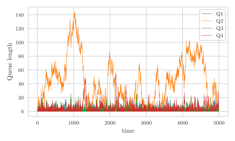
To gain insight into such systems, we simulate a chain of \(4\) stations in tandem, which means that jobs arrive at station 1, are then sent to station 2, etc., until they leave the network after station \(4\). Jobs neither visit the same server nor leave the network prematurely.
We simulate \(n=5000\) periods and take \(L_0^i=0\) at every station. The external arrivals at station 1 are independent and uniformly distributed on \(\{5,6,7\}\). The service capacities are independent, with
\begin{align*} c_k^1 &\sim \Pois{7}, & c_k^2 &\sim \Pois{6.1}, & c_k^3 &\sim \Pois{7.5}, & c_k^4 &\sim \Pois{7}. \end{align*}Thus, station 2 has the smallest mean service capacity.
Let \(a_k^1=a_k\), and for stations \(i=2,3,4\), let the arrivals be the departures from the preceding station. Since these downstream arrivals can be served in the same period, the tandem system satisfies
\begin{align*} a_k^1 &= a_k, & a_k^i &= d_k^{i-1},\\ d_k^i &= \min\{\L_{k-1}^i+a_k^i,c_k^i\}, & \L_k^i &= \L_{k-1}^i+a_k^i-d_k^i. \end{align*}Applying these recursions successively to the four stations produces Fig. 2.3. Station 2, which has the smallest mean service capacity, typically has the longest queue. This brings us to an interesting idea: to improve performance, invest in the bottleneck. In practice, identifying the bottleneck can be difficult because service capacities are hard to estimate.6The capacity may depend on the person at the station on a certain day. There can also be disturbances due to missing raw materials or machine breakdowns. In short, in practical situations, there are many messy details that disturb the assembly of high-quality data.
TF 1.
A general queueing system is stable when the arrival rate is not higher than the service rate.
Solution
Did you actually try? Write your solution down first for comparison.
Show the solution
False. The condition allows \(\lambda = \mu\), in which case stochastic queues are not stable.
TF 2.
If we find the average queue length too large, then we must increase the average service rate to decrease the average queue length.
Solution
Did you actually try? Write your solution down first for comparison.
Show the solution
False. We can also block jobs, or reduce the variability of the arrival or service process.
TF 3.
We consider a discrete-time queueing system with \(a_k\) the number of arrivals in period \(k\), and \(c_k\) the service capacity. Let \(d_k = \min\{L_{k-1}, c_k\}\), \(L_k = L_{k-1} -d_k + a_k\). Take \(a_k \sim \Pois{2}\), \(c_k\sim \Pois{1}\), and \(L_0 = 0\). Claim: \(\P{L_{1000} \geq 100} \leq 1/2\).
Solution
Did you actually try? Write your solution down first for comparison.
Show the solution
False. Since, on average, two jobs arrive per period and one leaves, the queue length increases on average by one job per period. After 1000 periods, the system must contain about 1000 jobs. As the Poisson distribution has a small relative variability (if \(X\sim \Pois{\lambda}\), then \(\V X / (\E X))^{2} = 1/\lambda\)), the probability that \(L_{1000}< 100\) is exceedingly small.
TF 4.
Claim: The scv of a rv \(X\) is the same as the scv of \(\alpha X\) if \(\alpha\) is a positive scalar.
Solution
Did you actually try? Write your solution down first for comparison.
Show the solution
True.
TF 5.
The parking meters at the universities are redesigned. A study has shown that the average amount of time individuals need to spend to pay for parking meters has decreased. Claim: As long as the inter-arrival distribution stays the same, the average queue length at the parking meter will be smaller.
Solution
Did you actually try? Write your solution down first for comparison.
Show the solution
False. Variability in payment time also affects the queue length.
TF 6.
Claim: When \(X \sim \Exp{\lambda}\) its scv exceeds 1.
Solution
Did you actually try? Write your solution down first for comparison.
Show the solution
False.
TF 7.
Consider a queue with an exponential inter-arrival distribution and a uniform service time distribution on \([0,A]\). Claim: \(C_s^2 = \frac{1}{3}\).
Solution
Did you actually try? Write your solution down first for comparison.
Show the solution
True.
Exercise 8.
A queueing system is under periodic review, that is, at the end of each period, the queue length is measured. Jobs arriving at period \(k\) cannot be served in period \(k\) and the system cannot contain more than \(K\) jobs; in other words, jobs are blocked when the system is too full. Develop recursions for \(\{L_k\}\), the number of jobs lost per period, and the fraction of jobs lost over \(T\) periods.
Solution
Did you actually try? Write your solution down first for comparison.
Show the solution
Jobs that would make the queue length exceed \(K\) are blocked. First, \(d_k\) jobs depart. Let \(\widetilde L_k\) be the queue length that would result after adding the new arrivals without blocking. The actual queue length is capped at \(K\), and the difference is the number of jobs lost:
\begin{align*} d_k &= \min\{\L_{k-1},c_k\}, & \widetilde L_k &= \L_{k-1}+a_k-d_k,\\ \L_k &= \min\{\widetilde L_k,K\}, & \ell_k &= \widetilde L_k-\L_k. \end{align*}Thus, the average number of jobs lost per period and the fraction of arrivals lost over \(T\) periods are, respectively,
\begin{align*} \overline\ell_T &= \frac{1}{T}\sum_{k=1}^{T}\ell_k, & q_T &= \frac{\sum_{k=1}^{T}\ell_k}{\sum_{k=1}^{T}a_k}. \end{align*}Exercise 9.
All items produced by a machine are tested. With probability \(p\) an item turns out to be defective and put at the head of the queue. The production time of new and faulty items is equal. Suppose that items cannot be served in the period in which they arrive, develop a set of recursions to simulate \(\{L_k\}\).
Hint
When the machine makes \(n\) items, and each of these is faulty with probability \(p\), then the number of faulty items is \(\Bin{n, p}\).
Solution
Did you actually try? Write your solution down first for comparison.
Show the solution
First, \(s_k\) items are processed. Of these, \(r_k\) are defective and return to the head of the queue, so only \(d_k=s_k-r_k\) items leave the system permanently. The queue update therefore subtracts only \(d_k\), which is how the defective items remain in the system. This gives the recursions
\begin{align*} s_k &= \min\{\L_{k-1},c_k\}, & r_k\mid s_k &\sim \Bin{s_k,p},\\ d_k &= s_k-r_k, & \L_k &= \L_{k-1}+a_k-d_k. \end{align*}An interesting challenge: Can you use these recursions to \emph{prove} that the long-run average service capacity \(n^{-1}\sum_{k=1}^n c_k\) must be larger than \(\gamma/(1-p)\), where \(\gamma = \lim_{n\to \infty} n^{-1}\sum_{k=1}^n a_k\) is the arrival rate of new jobs?
Exercise 10.
Sometimes items need re-work. Suppose a fraction \(p\) of items does not meet the quality requirements after the first pass at a machine, but requires a second pass to repair the problems. Assume that repair jobs need half the service time of new jobs and are served with priority over new jobs. Develop the recursions.
Hint
Make a queue for new and repaired items and use Exercise 4.
Solution
Did you actually try? Write your solution down first for comparison.
Show the solution
Let \(\L_k^R\) and \(\L_k^N\) be the numbers of repair and new jobs, respectively. Repair jobs have priority. Because a repair needs half the service time of a new job, one unit of capacity can process two repairs. We process repair jobs in pairs; if \(\L_{k-1}^R\) is odd, one repair waits for a later period. After the repairs, \(c_k^N\) is the capacity left for new jobs. Of the \(d_k^N\) new jobs processed, \(a_k^R\) require repair and join the repair queue for the next period. These modeling choices give the recursions
\begin{align*} d_k^R &= 2\min\left\{\left\lfloor\frac{\L_{k-1}^R}{2}\right\rfloor,c_k\right\}, & c_k^N &= c_k-\frac{d_k^R}{2},\\ d_k^N &= \min\{\L_{k-1}^N,c_k^N\}, & a_k^R &= \left\lfloor p d_k^N+\frac12\right\rfloor,\\ \L_k^R &= \L_{k-1}^R+a_k^R-d_k^R, & \L_k^N &= \L_{k-1}^N+a_k-d_k^N. \end{align*}As a general observation: there are many ways to organize the repairs. Do we serve them with priority or not, do we bin them and make new items instead, do we do the repairs on another, separate, station? Such differences should be reflected in a simulation model.
Exercise 11.
Consider a network with two production stations in tandem, i.e., all jobs from station 1 move on to station 2, and blocking, i.e., the server at station 1 is not allowed to produce more than the amount \(M\) station \(2\) can maximally contain. Assume that jobs moving from station 1 to station 2 arrive at the end of a period (hence cannot be served in that period), and must fit at the second station before any jobs from station 2 leave. Find recursions.
Hint
In addition to the regular conditions, we need to impose \(c^1_{k+1} \leq M-L^2_k\).
Solution
Did you actually try? Write your solution down first for comparison.
Show the solution
A first attempt would limit departures from station 1 by \(M-\L_{k-1}^2\), the free space at station 2. This quantity can be negative, for example when the initial queue at station 2 exceeds \(M\), so we use its positive part. Moreover, because transfers from station 1 must fit before station 2 serves any jobs, the available space is based on \(\L_{k-1}^2\), not on the queue after \(d_k^2\) departures. The complete recursions are
\begin{align*} d_k^1 &= \min\{\L_{k-1}^1,c_k^1,[M-\L_{k-1}^2]^+\}, & d_k^2 &= \min\{\L_{k-1}^2,c_k^2\},\\ \L_k^1 &= \L_{k-1}^1+a_k^1-d_k^1, & \L_k^2 &= \L_{k-1}^2+d_k^1-d_k^2. \end{align*}Exercise 12.
Consider the discrete-time model specified by (2.1.1). We assume that \(a_{k}\) is a \emph{batch} of jobs arriving in period \(k\) after the departures \(d_k\) have left. Give an estimator of \(\P{\L\leq m}\) for a situation in which the first job of the batch sees \(L_{k-1} - d_k\) jobs in the system, the second sees \(L_{k-1}-d_k + 1\) jobs, and so on.
Solution
Did you actually try? Write your solution down first for comparison.
Show the solution
Because departures occur before the batch arrives, first determine \(d_k\), then add \(a_k\) to obtain the new queue length. Thus,
\begin{align*} d_k &= \min\{\L_{k-1},c_k\}, & \L_k &= \L_{k-1}+a_k-d_k. \end{align*}The \(j\)th job in the batch arriving in period \(k\) sees \(\L_{k-1}-d_k+j-1\) jobs. Let \(N_T=\sum_{k=1}^{T}a_k\). Counting the arriving jobs that see at most \(m\) jobs in the system and dividing by the total number of arrivals gives an arrival-weighted empirical distribution, rather than a time average of the queue length:
\begin{align*} \widehat F_T(m) &=\frac{1}{N_T}\sum_{k=1}^{T}\sum_{j=1}^{a_k} \1{\L_{k-1}-d_k+j-1\leq m}. \end{align*}