2.2 Simulating the Psychiatrists Case

In the previous section, we showed how to analyze a case with five psychiatrists acting as five parallel servers processing a queue of patients waiting for an intake. Moreover, we proposed a good rule to control the queue length. In this section, we discuss the algorithms used to produce Fig. 2.1.

Before accounting for holidays, the weekly capacities of the five psychiatrists under the unbalanced and balanced plans are, respectively,

\begin{align*} b^u &= (1,1,1,3,9), & b^b &= (2,2,3,4,4). \end{align*}

To make the case with unbalanced capacity and spread holidays, we take

\begin{align*} c_{i,k}^{\mathrm{spread}} &=b_i^u\1{i\neq1+((k-1)\bmod5)}. \end{align*}

For the case with unbalanced capacity and synchronized holidays, we take

\begin{align*} c_{i,k}^{\mathrm{sync}} &=b_i^u\1{(k-1)\bmod5\neq0}. \end{align*}

The corresponding balanced schemes are obtained by replacing \(b^u\) in the two expressions above by \(b^b\). In what follows, let \(c_{i,k}\) denote the capacity of psychiatrist \(i\) in week \(k\) for any one of these four scenarios.

We simulate \(n=1000\) weeks, with independent weekly arrivals \(a_k\sim\Pois{11.8}\). For each capacity scenario, the initial queue length is \(L_0=0\), and the total capacity in week \(k\) is \(c_k=\sum_{i=1}^{5}c_{i,k}\). Combining the balanced and unbalanced plans with the spread and synchronized holiday patterns gives four capacity scenarios. Applying Alg. 2.2.1 to each scenario produces the trajectories in the left panel of Fig. 2.1.

\begin{algorithm}
\caption{Compute the queue lengths.}
\begin{algorithmic}[1]
\State \textbf{Input:} arrivals \((a_1,\ldots,a_n)\), capacities \((c_1,\ldots,c_n)\), and initial queue length \(L_0\)
\State \textbf{Output:} queue lengths \((L_1,\ldots,L_n)\)
\For{\(k=1,\ldots,n\)}
    \State \(d_k\gets\min\{L_{k-1}+a_k,c_k\}\)
    \State \(L_k\gets L_{k-1}+a_k-d_k\)
\EndFor
\Return \((L_1,\ldots,L_n)\)
\end{algorithmic}

\end{algorithm}

For the controlled system in the right panel of Fig. 2.1, we use the capacity rule in (2.1.7). Alg. 2.2.2 implements the resulting simulation. We apply the control rule separately with \(e=1\), \(e=2\), and \(e=5\). The resulting trajectories are shown in the right panel of Fig. 2.1.

\begin{algorithm}
\caption{Simulate the queue with state-dependent capacity.}
\begin{algorithmic}[1]
\State \textbf{Input:} arrivals \((a_1,\ldots,a_n)\), control size \(e\), and initial queue length \(L_0\)
\State \textbf{Output:} queue lengths \((L_1,\ldots,L_n)\)
\For{\(k=1,\ldots,n\)}
    \If{\(L_{k-1}\geq48\)}
        \State \(c_k\gets12+e\)
    \ElsIf{\(L_{k-1}\leq24\)}
        \State \(c_k\gets12-e\)
    \Else
        \State \(c_k\gets12\)
    \EndIf
    \State \(d_k\gets\min\{L_{k-1}+a_k,c_k\}\)
    \State \(L_k\gets L_{k-1}+a_k-d_k\)
\EndFor
\Return \((L_1,\ldots,L_n)\)
\end{algorithmic}

\end{algorithm}

The next true-false questions and exercises relate to the \(N\)-policy.

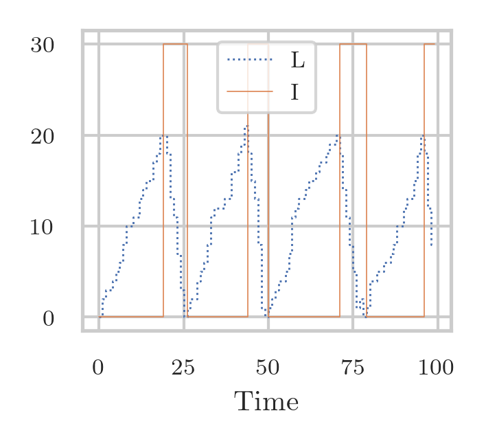In the queueing systems we have analyzed up to now, the server is always present to start serving jobs at the moment they arrive.¹¹A queue under an \(N\)-policy. . However, in cases in which there is a significant cost associated with changing the server from idle to busy this condition is typically not satisfied. To reduce the average cost, we can use an \(N\)-policy, which works as follows.²²\(N\)-policies are used to decide when to heat up a large oven.