5.4 M/G/1 Queue: Expected Waiting Time

The Pollaczek-Khinchine (PK) formula for the average waiting time of an \(M/G/1\) queue is a key result in Operations Research. We derive it using the renewal reward theorem, and follow the steps of Section 5.3.

We start from the simple observation that before an arrival gets access to the server, it must first wait for the job in service¹¹If any. to complete, then for the queue to clear. From PASTA it follows that \(\E{\W} = \E{S_r} + \E{\QQ} \E S\), where \(\E{S_r}\) is the (time-)average remaining service time of the job in service.²²The rv \(S_{r}\) is also known as the remaining lifetime and is widely used in maintenance theory and actuarial sciences. With Little’s law \(\E \QQ = \lambda \E\W\) and \(\rho = \lambda \E S\),

\begin{equation*} \E \W = \E{S_{r}} + \lambda \E \W \E S \implies \E{\W} = \frac{\E{S_r}}{1-\rho}. \tag{5.4.1} \end{equation*}

To proceed, we need an expression for \(\E{S_r}\).

Theorem 5.4.1.

The expected remaining service time as observed by Poisson arrivals is

\begin{equation*} \E{S_r} = \frac{\lambda}2 \E{S^2}, \end{equation*}

provided the second moment of \(S\) exists.

Proof

In Fig. 5.1, the service of job \(k\) starts at \(\As_{k}\), so the job departs at time \(D_k=\As_k + S_k\). Hence, at any time \(s \in [\As_{k}, D_{k}]\), the remaining service time of job \(k\) is \(D_k-s\).

from pathlib import Path
import sys
sys.path.insert(0, str((Path.home() / "vakken" / "course-common" / "scripts").resolve()))
from render_tikz import render_tikz

render_tikz(r"""
\begin{tikzpicture}[scale=1,
 open/.style={shape=circle, fill=white, inner sep=1pt, draw, node contents=},
 closed/.style={shape=circle, fill=black, inner sep=1pt, draw, node contents=}]
 \draw (-1,0) -- (4,0);
 \draw node (c1) at (0,3) [closed, label={}]
 node (c2) at (3,0)[open, label={}]
 (c1) to (c2);
 \draw[dotted] (0,0) -- (0,3) node[midway, rotate=90, fill=white] {$S_k$};
 \node[below] at (0,0) {$\As_k$};
 \node[below] at (3,0) {$D_k$};
 \draw[<->, dotted] (0.75,0) -- (0.75,2.25) node[midway,fill=white,rotate=90] {$D_k-s$};
 \node[below] at (0.75,0) {$s$};
\end{tikzpicture}
""", "../figures/mg1_remaining_service.png")

⊕
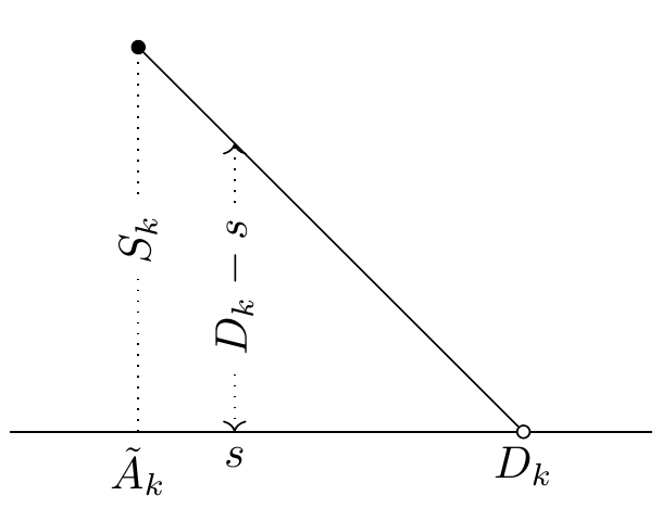
Figure 5.1: Remaining service time.

More generally, at some arbitrary time \(s\), the number of departures is \(D(s)\). Thus, \(D(s)+1\) is the index of the first job to depart after time \(s\), and its departure time is \(D_{D(s)+1}\). Consequently, the remaining service time at time \(s\) is \(D_{D(s)+1}-s\), provided that this job is in service, i.e., \(\As_{D(s)+1} \leq s\). The total remaining service time as seen by the server up to time \(t\) is therefore

\begin{equation*} R(t) = \int_0^t (D_{D(s)+1}-s)\1{\As_{D(s)+1} \leq s} \d s, \end{equation*}

and \(\lim_{t\to\infty} R(t)/t = \E{S_{r}}\).

In Fig. 5.1, \(R(D_k) - R(D_{k-1}) =:Z_k\) equals the area of the triangle. By inspecting \(R(\cdot)\) at \(\{D_{k}\}\), we see that \(Z=\lim_{n\to\infty} \frac{1}{n}\sum_{k=1}^n S_k^2/ 2 = \E{S^2}/2\). By the renewal-reward theorem, \(R=\delta Z\), but \(\delta = \lambda\) by rate-stability. The claim follows now from PASTA.

Noting that

\begin{equation*} \frac{\E{S^2}}{(\E S)^2} = \frac{\E{S^2} - (\E S)^{2} + (\E{S})^{2}}{(\E S)^2} = \frac{\V S + (\E S)^{2}}{(\E S)^{2}} = C_s^2 +1. \end{equation*}

and substituting this in the expression for \(\E{S_{r}}\) we obtain from (5.4.1) the following result.

Theorem 5.4.2.

The expected waiting time in the \(M/G/1\) queue equals³³The Pollaczek-Khinchine (PK) formula.

\begin{equation*} \E{\W} = \frac 1 2 \frac{\lambda \E{S^2}}{1-\rho} =\frac{1 + C_s^2}2 \frac{\rho}{1-\rho} \E S. \tag{5.4.2} \end{equation*}

The Pollaczek-Khinchine equation can also be found as a limiting case of the waiting time of the \(M^{B}/M/1\) queue by interpreting a job in the \(M/G/1\) as a batch consisting of many tiny items in the \(M^{B}/M/1\) queue.⁴⁴If you are not interested in math, you may skip the next derivation. Suppose that in the \(M^{B}/M/1\) queue the service times of the items are iid with mean \(1/\nu\). If \(F\) is the cdf of the service times of the \(M/G/1\) queue, then we take

\begin{equation*} \P{B=k} = F(k/\nu) - F((k-1)/\nu) \end{equation*}

as the probability that a batch has size \(k\) in an \(M^{B}/M/1\) queue. Note that in the \(M^{B}/M/1\) queue, when a batch has size \(k\), the service time is the sum of \(k\) rvs that are \(\Exp{\nu}\); thus, the service time of a batch of size \(k\) is \(\sim \Gamm{k, \nu}\). When \(\nu \gg 1\), the expected service time of a batch is

\begin{align*} \E{S_{B}} &= \E{\E{S_{B}|B}} = \E{\frac{B}{\nu}} = \sum_{k=0}^{\infty} \frac{k}{\nu} \P{B=k} \\ &= \sum_{k=0}^{\infty} \frac{k}{\nu} \qb{F\rb{\frac{k}{\nu}} - F\rb{\frac{k-1}{\nu}}} \approx \int_{0}^{\infty} x \d F(x) = \E S. \end{align*}

In words, when \(\nu\) is large, the batch expected service time in an \(M^{B}/M/1\) queue approximates the expected service time in an \(M/G/1\) queue.

In fact, the proof that the expected waiting time of the \(M^{B}/M/1\) converges to the Pollaczek-Khinchine equation when \(\nu\to \infty\) is based on the fact that every cdf \(F\), concentrated on \([0, \infty)\), can be approximated (weakly) by the sequence of cdfs⁵⁵See Asmussen, Section III.4, Applied Probability and Queues, 2003.

\begin{equation*} F_{\nu}(x) = F(0) + \sum_{k=1}^{\infty} \qb{F\rb{\frac k \nu} - F\rb{\frac{k-1}\nu}} \int_0^x \frac{\nu^k t^{k-1}}{(k-1)!} e^{-\nu t} \d t,\quad\text{as } \nu\to\infty. \end{equation*}

That is, the distribution of the service time of a batch whose items have \(\Exp{\nu}\) service times approaches the cdf \(F\) of the service time of the \(M/G/1\) queue. Thus, when \(\nu\to\infty\) in (5.3.4), the mean and scv of the batch service time converge to \(\E S\) and \(C_{S}^{2}\) of the job, and the last term vanishes as it is proportional to \(1/\nu\). This leads to (5.4.2).

TF 1.

Consider the \(M/G/1\) queue. Denote by \(\tilde{A}_k\) the time job \(k\) starts service and by \(D_k\) its departure time, \(k=1,\ldots,n\). Claim: the expression

\begin{equation*} \sum_{k=1}^{n} \int_0^{D_n} (D_k-s)\1{\As_k \leq s < D_k} \d s \end{equation*}

represents the total remaining service time up to \(t = D_n\).

Solution

Did you actually try? Write your solution down first for comparison.

Show the solution

True.

TF 2.

Claim: For an \(M/D/1\) queue, \(\E{\W}=\frac{\rho}{1-\rho}\frac{\E{S}}{2}\).

Solution

Did you actually try? Write your solution down first for comparison.

Show the solution

True.

TF 3.

Claim: The PK formula shows that \(\E\W\) is linear in \(\rho\).

Solution

Did you actually try? Write your solution down first for comparison.

Show the solution

False. The factor \(\rho/(1-\rho)\) makes \(\E\W\) a nonlinear, convex function of \(\rho\) that diverges as \(\rho\uparrow 1\).

TF 4.

Claim: For the \(M/G/1\) queue, the expected remaining service time \(\E{S_r}\) does not depend on the service time distribution, only on \(\E S\).

Solution

Did you actually try? Write your solution down first for comparison.

Show the solution

False. \(\E{S_r} = \lambda \E{S^2}/2\), which depends on the second moment of the service time, not just the mean.

TF 5.

Claim: The derivation of the PK formula uses both PASTA and Little’s law.

Solution

Did you actually try? Write your solution down first for comparison.

Show the solution

True. PASTA is used to conclude that \(\E\W = \E{S_r} + \E\QQ \E S\), and Little’s law to replace \(\E\QQ\) by \(\lambda \E\W\).

Exercise 6.

Consider a workstation with only one machine. We model the job arrival process as a Poisson process with rate \(\lambda=3\) per day. The average service time \(\E S = 2\) hours, \(C^2_s = 1/2\), and the store operates 8 hours per day. Show that \(\E{\W} = 4.5\) h. What would you propose to reduce \(\E \W\) to 2h?

Solution

Did you actually try? Write your solution down first for comparison.

Show the solution

Expressing the arrival rate per hour gives

\begin{align*} \lambda &= \frac{3}{8}, & \rho &= \lambda\E S=\frac{3}{8}\,2=\frac34. \end{align*}

Since the arrivals are Poisson, \(C_a^2=1\). Substitution in the waiting-time formula gives \[ \E W =\frac{C_a^2+C_s^2}{2}\frac{\rho}{1-\rho}\E S =\frac{1+1/2}{2}\frac{3/4}{1/4}\,2 =4.5\text{ hours}. \]

Eliminating all service-time variability is not sufficient. Indeed, when \(C_s^2=0\), \[ \E W=\frac12\frac{3/4}{1/4}\,2=3\text{ hours}. \] Thus, capacity must also be increased, for instance by adding another machine or reducing the average service time. As an illustration, if \(\E S=1\) hour and \(C_s^2=1/3\), then \(\rho=3/8\) and \[ \E W =\frac{1+1/3}{2}\frac{3/8}{5/8}\,1 =0.4\text{ hours}. \]

Exercise 7.

Compare the expected waiting times in the \(M/D/1\) and the \(M/M/1\) queues.

Hint

Use \(\V S=0\) for the \(M/D/1\) queue and \(C_{s}^{2} = 1\) for the \(M/M/1\) queue.

Solution

Did you actually try? Write your solution down first for comparison.

Show the solution

\(\V S = 0 \implies C_s^2 = 0 \implies \E{\W_{M/D/1}} = {\E{\W_{M/M/1}}}/2\).

Exercise 8.

Compute \(\E\J\) for the \(M/G/1\) queue with \(S\sim U[0,\alpha]\).

Solution

Did you actually try? Write your solution down first for comparison.

Show the solution

\begin{align*} \E S &= \alpha/2, & \E{S^2} &= \frac{1}{\alpha}\int_0^\alpha x^2 \d x = \alpha^2/3,\\ \V S &= \alpha^2/3 - \alpha^2/4= \alpha^2/12, & C_s^2 &= (\alpha^2/12)/(\alpha^2/4) = 1/3,\\ \rho &= \lambda \alpha/2,\\ \E{\W} &= \frac{1+C_s^2}2 \frac{\lambda \alpha/2}{1-\lambda \alpha/2}\frac \alpha2, & \E \J &= \E{\W} + \frac \alpha2. \end{align*}

Exercise 9.

Show that for the \(M/G/1\) that \(\E{S_r} = \rho \E{S_r\given S_r>0}\). As a consequence, for the \(M/M/1\) queue, \(\E{S_{r}} \neq \E S\). Why not?

Hint

Use the PASTA property. Note that when estimating \(\E{S_r}\) along a sample path, \(S_r=0\) for jobs that arrive at an empty system.

Solution

Did you actually try? Write your solution down first for comparison.

Show the solution

The probability of finding the server busy upon arrival is \(\rho\), and only arrivals that find the server busy observe \(S_r>0\).

\begin{equation*} \E{S_r} = \rho \E{S_r\given S_r >0} + (1-\rho) \E{S_r\given S_r = 0} = \rho \E{S_r\given S_r>0}. \end{equation*}

For the \(M/M/1\), service times are memoryless, so \(\E{S_r \given S_r>0} = \E S\), which implies \(\E{S_r} = \rho \E S\) for the \(M/M/1\) queue.

5.4 \(M/G/1\) Queue: Expected Waiting Time