5.3 M^B/M/1 Queue and Rejection Policies

In this section, by using the renewal-reward theorem, we derive for the \(M^{B}/M/1\) queue expressions for \(\rho\), \(\E \W\), and \(\E \L\). To compute more difficult performance measures, such as the loss probability \(\P{\L>n}\), we need expressions for the stationary distribution \(\pi(n)\). We use level-crossing to derive a recursive scheme which, when combined with a policy to reject batches, can be used to compute these probabilities.

Assume that batches arrive as a Poisson process with rate \(\lambda_{B}\), and the number of jobs in a batch are iid \(\sim B\). Let \(S_{k,i}\) denote the service time of the \(i\)th job of batch \(k\); assume that the \(S_{k, i}\) are iid \(\sim S\) and independent of \(B\). By (4.1.2) the utilization \(\rho = \lambda_{B} \E B \E S\); as always, we require \(\rho<1\).

An arriving batch joins the end of the queue (if present). Once it arrives at the head of the queue, the batch moves in its entirety to the server¹¹This is the same batching model as in Section 6.2., and then the server processes the jobs one after another until the batch is finished. Writing \(\QQ^B\) for the number of batches in queue and \(\Ls^B\) for the number of jobs (if any) at the server, the average time \(\E{\W^{B}}\) a batch spends in queue is²²First the jobs at the server have to be served, then the ones in queue.

Substituting the equality³³Little’s law. \(\E{\QQ^B} = \lambda_{B} \E{\W^B}\) and simplifying yields

We can relate the average time \(\E \W\) a job spends in queue to \(\E{\W^{B}}\) by observing that \(\E{\Ls^B} + \E{\QQ^B} \E B = \E \L\),⁴⁴The total number of jobs in the system is the number at the server plus the number in queue. The latter equals the number of batches in queue times the average batch size. so from (5.3.1)

where 1 follows from the memorylessness of the service time of the job in service (if any). Thus, to compute \(\E \W\) it remains to find an expression for \(\E{\Ls^B}\) in (5.3.2).

For this, we use the renewal reward theorem. Define⁵⁵Much like the proof of Little’s law. \(R(t) := \int_0^t \Ls^B(s) \d s\), where \(\Ls^{B}(s)\) is the number of jobs (of the batch in service) at the server at time \(s\), and \(Z_k = R(D_k)-R(D_{k-1})\) where \(D_k\) is the departure time of the \(k\)th batch. Suppose the \(k\)th batch has batch size \(B_{k}\), then

because \(B_{k}\) jobs are at the server during the service of the first job, \(B_{k}-1\) during the service of the second, \ldots Using that the \(S_{k,i} \sim S\),

As \(B_{k}\sim B\),

We now have all elements to fill in \(R=\alpha Z\). First, \(R = \lim_{t\to\infty}R(t)/t = \E{L_{S}^{B}}\). Second, we sample at batch departure moments, so \(\alpha=\delta_{B}\) which equals \(\lambda_{B}\) by rate stability. Third, \(Z=\E{Z_{k}}\). Combining all this, and using that \(\rho=\lambda_{B} \E B\E S\), we obtain

We can brush this up by realizing that⁶⁶Recall that the scv of a rv \(B\) is \(C_B^2 = \V B/ (\E B)^{2}\). We assume that \(\E{B^{2}} < \infty\).

Substituting this into the above gives the final result

This formula is an important result. It tells us that \(\E \W\) increases when the load \(\rho\) or the variability \(C_{B}^{2}\) or \(\E B\) or \(\E S\) increases (even when the utilization \(\rho\) remains the same). As such, it gives us the most important clues about what to change if \(\E \W\)⁷⁷Hence, by Little’s law, \(\E \L\). has to be reduced.

Rather than using the time an entire batch spends at the server, we can concentrate on the expected time spent by a single job at the server. This will provide us with a simple expression for \(\P{\Ls^{B}=i}\), from which we also can derive (5.3.3).

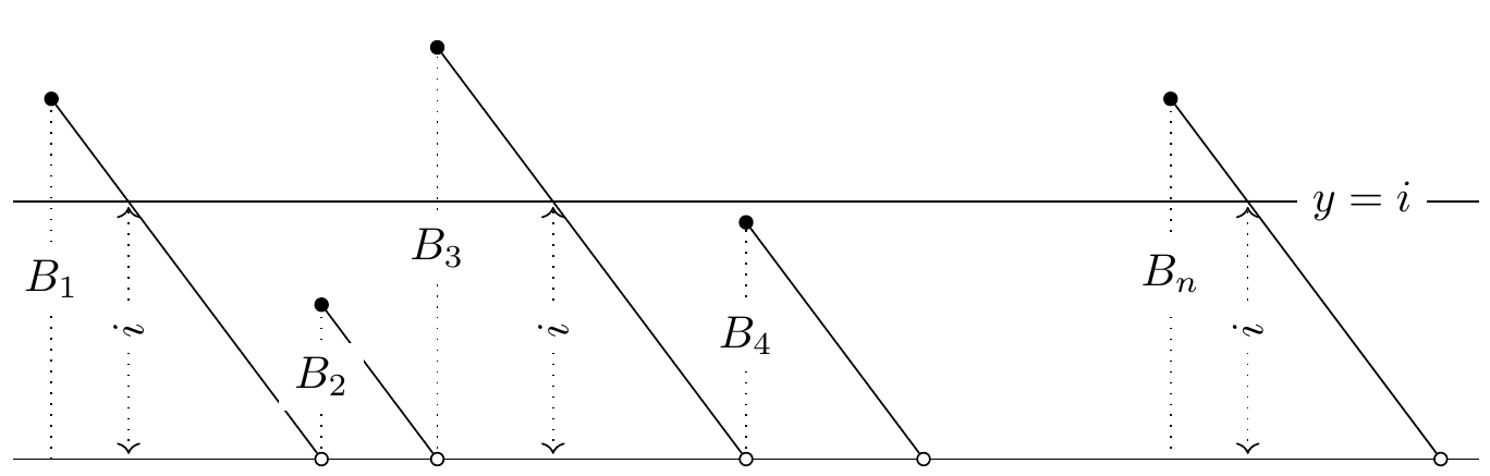
In this case, let \(R_i(t) = \int_0^t \1{\Ls^{B}(s)=i} \d s\) be the total time there are \(i\) jobs at the server, so that \(R_i(t)/t \to \P{\Ls^{B}=i}\) as \(t\to\infty\). By sampling \(R(\cdot)\) at batch departure times \(\{D_k\}\), see Fig. 5.1, we see that

because only when \(B_{k}\geq i\), we can see \(i\) jobs at the server for the \(k\)th batch, and then \(S_{k,i}\) is the time this job occupies the server. With this,

since \(S_{k, i}\) and \(B_{k}\) are independent, and⁸⁸Recall: \(\P{A} := \E{\1{A}}\). \(G(i-1) = \E{\1{B\geq i}} = \P{B> i-1}\) is the survivor function of \(B\). With the renewal reward theorem and rate stability, \(\delta_{B} = \lambda_{B}\), we conclude that

This expression provides us with another derivation of (5.3.4). Just note that \(\E{\Ls^{B}} = \sum_{i=0}^\infty i \P{\Ls^{B}=i} = \lambda_{B} \E S \sum_{i=1}^\infty i G(i-1)\) and use Exercise 12 to simplify.

from pathlib import Path
import sys
sys.path.insert(0, str((Path.home() / "vakken" / "course-common" / "scripts").resolve()))
from render_tikz import render_tikz

render_tikz(r"""
\begin{tikzpicture}[yscale=0.8,xscale=0.6,
 open/.style={shape=circle, fill=white, inner sep=1pt, draw, node contents=},
 closed/.style={shape=circle, fill=black, inner sep=1pt, draw, node contents=}]

 % y = zero line
 \draw (-0.5, 0) -- (18.5, 0);
 % level crossing
 \draw (-0.5, 2.5) -- (18.5, 2.5)
 node[pos=0.92, fill=white] {$y=i$};

 \draw node (c1) at (0,3.5) [closed, label={}]
 node (c2) at (3.5,0)[open, label={}]
 (c1) to (c2);
 \draw[dotted] (0,0) -- (0,3.5) node[midway, fill=white] {$B_1$};
 \draw[dotted, <->] (1, 0.05) -- (1, 2.45) node[fill=white, midway, rotate=90] {$i$};

 \draw node (c1) at (3.5,1.5) [closed, label={}]
 node (c2) at (5,0)[open, label={}]
 (c1) to (c2);
 \draw[dotted] (3.5,0.1) -- (3.5,1.5) node[midway, fill=white] {$B_2$};

 \draw node (c1) at (5,4) [closed, label={}]
 node (c2) at (9,0)[open, label={}]
 (c1) to (c2);
 \draw[dotted] (5,0.1) -- (5,4) node[midway, fill=white] {$B_3$};
 \draw[dotted, <->] (6.5, 0.05) -- (6.5, 2.45) node[fill=white, midway, rotate=90] {$i$};

 \draw node (c1) at (9,2.3) [closed, label={}]
 node (c2) at (11.3,0)[open, label={}]
 (c1) to (c2);
 \draw[dotted] (9,0.1) -- (9,2.3) node[midway, fill=white] {$B_4$};

 % end
 \draw node (c1) at (14.5,3.5) [closed, label={}]
 node (c2) at (18,0)[open, label={}]
 (c1) to (c2);
 \draw[dotted] (14.5,0.1) -- (14.5,3.5) node[midway, fill=white ] {$B_n$};
 \draw[dotted, <->] (15.5, 0.05) -- (15.5, 2.45) node[fill=white, midway, rotate=90] {$i$};

\end{tikzpicture}
""", "../figures/batch_remaining_service.png")

The second task is to use level-crossing to find a recursive formula for the state probabilities \(\{\pi(n)\}\).⁹⁹Note: \(n\) means the number of jobs in the system, not the number of batches. For this we need to generalize our earlier level-crossing equation \(\lambda p(n) = \mu p(n-1)\) because when a batch arrives, multiple levels can be up-crossed, see Fig. 5.2. We use the PASTA property to express level-crossing in terms of \(\{\pi(n)\}\) instead of \(\{p(n)\}\).

from pathlib import Path
import sys
sys.path.insert(0, str((Path.home() / "vakken" / "course-common" / "scripts").resolve()))
from render_tikz import render_tikz

render_tikz(r"""
\begin{tikzpicture}[scale=1,
 >=stealth',
 circ/.style={
 circle,
 draw=black,
 thick,
 minimum size=1.cm,
 inner sep=0pt,
 text centered
 },
 pil/.style={
 ->,
 thick,
 shorten <=2pt,
 shorten >=2pt}
]

\draw[dashed, thick] node at (5,-1.5) [below] {level~$n$}
(5,-1.5) -- (5,3);

\node[circ] (n-2) {$n-2$};
\node[circ, right=of n-2] (n-1) {$n-1$};

\node[circ, right=of n-1] (n) {$ n $}
 edge[pil,<-, bend left=45] node[below] {$\lambda f(1)$} (n-1.south east);
\node[circ, right=of n] (n+1) {$n+1$}
 edge[pil,bend left=45] node[midway, fill=white] {$\mu$} (n.south east);
\node[above=of n+1] (inf) {}
 edge[pil, <-, bend right=45] node[midway, fill=white] {$\lambda G(0)$} (n.north east)
 edge[pil, <-, bend right=45] node[midway, fill=white] {$\lambda G(1)$} (n-1.north east)
 edge[pil, <-, bend right=45] node[midway, fill=white] {$\lambda G(2)$} (n-2.north east)
;
\end{tikzpicture}
""", "../figures/batch_level_crossing.png")

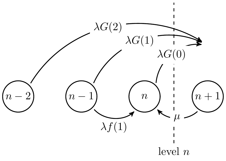
The down-crossing rate of level \(n\) is easy: since jobs are still served one-by-one, we have \(\mu \pi(n+1)\).

For the up-crossings of level \(n\) we should consider batch arrivals that see \(m\leq n\) jobs in the system. Since batches arrive at a rate \(\lambda_{B}\), PASTA implies that \(\lambda_{B} \pi(m)\) is the arrival rate of batches that see \(m\) upon arrival.¹⁰¹⁰That is, the total arrival process is thinned with a fraction \(\pi(m)\). When an arriving batch sees \(m\) jobs in the system, and level \(n\) has to be up-crossed, the batch must contain more than \(n-m\) jobs. As \(G(n-m)\) is the probability that the batch size is larger than \(n-m\) and as batch sizes are independent of arrival times, such batches arrive as a Poisson process with rate \(\lambda_{B} \pi(m) G(n-m)\). Finally, to compute the rate at which level \(n\) is up-crossed, we merge all these thinned Poisson processes into a new Poisson process with rate \(\lambda_{B} \sum_{m=0}^n \pi(m) G(n-m)\).

By level-crossing, the up-crossing and down-crossing rates must match, thus,

It is an important check¹¹¹¹Exercise 13. to retrieve (5.3.4) from the expression \(\E\L = \sum_{n} n \pi(n)\) and Little’s law.

It remains to find the normalization constant for \(\pi\). However, this is not possible in general because (5.3.5) does not lead to a closed form expression for \(\pi(n)\).¹²¹²Compare (5.1.1). Numerically, though, we can start with \(\pi(0)=1\), apply the recursion, and truncate when the (unnormalized) probabilities become negligible. For a bounded batch size, let \(K_B\) be its largest possible value. The procedure below first computes at least \(K_B\) values, so that it does not stop during an initial increase. It then continues until the unnormalized weights become negligible and finally normalizes them.

\begin{algorithm}
\caption{Compute the stationary probabilities of an \(M^B/M/1\) queue.}
\begin{algorithmic}[1]
\State \textbf{Input:} rates \(\lambda_B,\mu\), survivor function \(G\), largest batch size \(K_B\), threshold \(\epsilon\)
\State \textbf{Output:} the stationary-probability map \(\pi\)
\Procedure{BatchStationary}{\(\lambda_B,\mu,G,K_B,\epsilon=10^{-10}\)}
    \State \(q\gets\pr{Map}()\), \(q(0)\gets1\), \(n\gets0\)
    \While{\(n<K_B\) or \(q(n)>\epsilon\)}
        \State \(q(n+1)\gets\dfrac{\lambda_B}{\mu}\pr{Sum}\rb{\qb{q(m)G(n-m):m=0,\ldots,n}}\)
        \State \(n\gets n+1\)
    \EndWhile
    \State \(\pi\gets\pr{NormalizeMap}(q)\)
    \State \Return \(\pi\)
\EndProcedure
\end{algorithmic}

\end{algorithm}

A different approach is to completely bypass the normalization problem by blocking the demand above some level \(K\). There are three common policies for deciding which jobs in a batch to accept.

1. Complete acceptance: accept all batches that arrive when the system contains \(K-1\) or fewer jobs, and reject the entire batch when the system contains \(K\) or more jobs. For this case, we make the assumption that the batch size is bounded by the number \(K_{B}\) so that \(L(t) \leq K-1 + K_{B}\).¹³¹³Exercise 8.
2. Partial acceptance: accept whatever fits of a batch, i.e., up to \(K\), and reject the rest.¹⁴¹⁴Exercise 9.
3. Complete rejection: if a batch does not fit entirely into the system, reject it completely.¹⁵¹⁵Exercise 10.

In Exercise 9--Exercise 10 we will derive recursions similar to (5.3.5) to compute \(\{\pi(n)\}\) for these different blocking models.

\begin{algorithm}
\begin{algorithmic}[1]
\Procedure{CompleteRejection}{\(K,\lambda_B,\mu,G\)}
    \State \(q\gets\pr{Map}()\), \(q(0)\gets1\)
    \For{\(n=0,\ldots,K-1\)}
        \State \(q(n+1)\gets\dfrac{\lambda_B}{\mu}\pr{Sum}\rb{\qb{q(m)[G(n-m)-G(K-m)]:m=0,\ldots,n-1}}\)
    \EndFor
    \State \Return \(\pr{NormalizeMap}(q)\)
\EndProcedure
\end{algorithmic}

\end{algorithm}

Suppose \(B\) is geometrically distributed¹⁶¹⁶Sometimes this distribution is called the First Success distribution. There is no consensus on the definition of the geometric distribution, see Wikipedia. with \(\E B = 1/p\).

\begin{algorithm}
\caption{Compute the stationary probabilities under complete acceptance.}
\begin{algorithmic}[1]
\Procedure{CompleteAcceptance}{\(K,\lambda_B,\mu,G,K_B\)}
    \State \(q\gets\pr{Map}()\), \(q(0)\gets1\)
    \For{\(n=0,\ldots,K+K_B-2\)}
        \State \(M\gets\min\{n,K-1\}\)
        \State \(q(n+1)\gets\dfrac{\lambda_B}{\mu}\pr{Sum}\rb{\qb{q(m)G(n-m):m=0,\ldots,M}}\)
    \EndFor
    \State \Return \(\pr{NormalizeMap}(q)\)
\EndProcedure
\end{algorithmic}

\end{algorithm}

\begin{algorithm}
\caption{Compute the stationary probabilities under partial acceptance.}
\begin{algorithmic}[1]
\Procedure{PartialAcceptance}{\(K,\lambda_B,\mu,G\)}
    \State \(q\gets\pr{Map}()\), \(q(0)\gets1\)
    \For{\(n=0,\ldots,K-1\)}
        \State \(q(n+1)\gets\dfrac{\lambda_B}{\mu}\pr{Sum}\rb{\qb{q(m)G(n-m):m=0,\ldots,n}}\)
    \EndFor
    \State \Return \(\pr{NormalizeMap}(q)\)
\EndProcedure
\end{algorithmic}

\end{algorithm}

\begin{algorithm}
\caption{Compute the stationary probabilities under complete rejection.}
\begin{algorithmic}[1]
\Procedure{CompleteRejection}{\(K,\lambda_B,\mu,G\)}
    \State \(q\gets\pr{Map}()\), \(q(0)\gets1\)
    \For{\(n=0,\ldots,K-1\)}
        \State \(q(n+1)\gets\dfrac{\lambda_B}{\mu}\pr{Sum}\rb{\qb{q(m)[G(n-m)-G(K-m)]:m=0,\ldots,n}}\)
    \EndFor
    \State \Return \(\pr{NormalizeMap}(q)\)
\EndProcedure
\end{algorithmic}

\end{algorithm}

pi = mxm1()
print(pi.mean())

pi = complete_rejection(5)
print(pi.mean())
pi = partial_acceptance(5)
print(pi.mean())
pi = complete_acceptance(5)
print(pi.mean())