5.2 Applications of the M(n)/M(n)/1 queueing model
5.2 Applications of the \(M(n)/M(n)/1\) queueing model
In this section we apply the tools developed above to a number of interesting queueing systems. First, we discuss how to use the \(M(n)/M(n)/1\) queue to organize a part of a production process. Second, we show how to plan the number of servers at a call center such that the average queue length remains small.
Riley is an operations manager at a factory that produces custom metal parts for various industries. Riley’s factory has a single heat treatment furnace to temper the metal parts. Recently, Riley noticed an increase in customer orders, leading to long delays and dissatisfied clients.
- Should Riley sometimes block jobs to control the waiting time?
- Should Riley buy another oven to increase the capacity?
- If Riley bought a second oven, the utilization of both ovens may become quite low. However, as an oven is costly to heat up, it may be favorable to only switch on a second oven when queues are long.
To compare the effect of these different strategies, Riley hires us to model the operation of the oven using queueing theory. We consider the following metrics: average job waiting times, average number of jobs in the system, machine utilization, and job acceptance rate. For ease1At a later stage we can make more complicated models., we assume that jobs arrive as a Poisson process with a rate \(\lambda\) jobs per hour, and production times are \(\sim \Exp{\mu}\) with \(1/\mu = \E S\).
We implemented the level-crossing recursions and the KPI formulas from the previous section for each choice of the arrival and service rates. For the numerical comparison, take \(\lambda=1.9\) and \(\mu=2\) per hour. The results are as follows. Here, \(\bar\lambda\) is the acceptance rate and \(\rho\) is the capacity utilization.
| Policy | \(\E W\) | \(\E L\) | \(\bar\lambda\) | \(\rho\) | Loss |
|---|---|---|---|---|---|
| One oven | 9.50 | 19.00 | 1.90 | 0.95 | 0.00 |
| Capacity \(K=10\) | 2.04 | 4.49 | 1.77 | 0.88 | 0.07 |
| Two ovens | 0.15 | 1.23 | 1.90 | 0.47 | 0.00 |
| Controlled two ovens | 0.79 | 2.46 | 1.90 | 0.47 | 0.00 |
With one oven, the high utilization leads to a long expected waiting time. Limiting the system to \(K=10\) reduces the expected waiting time considerably, at the cost of rejecting about \(7\%\) of the jobs. Keeping two ovens running makes the expected waiting time almost negligible, but leaves much capacity unused. Switching on the second oven only when \(n\geq5\) provides a compromise: the expected waiting time is \(0.79\), while the first and second ovens are busy \(81\%\) and \(14\%\) of the time, respectively.
As a numerical check, increasing \(K\) from \(10\) to \(1000\) recovers the results of the \(M/M/1\) model without blocking.
Let us next discuss an example of employee planning at a call center. Here we keep the models simple, but we include all necessary steps to solve a realistic planning problem.
We start with specifying the arrival process. It is reasonable to model it as a Poisson process, as there are many potential customers, each choosing with a small probability of calling at a certain moment in time. Thus, we only have to characterize the arrival rate. Estimating this for a call center is easy because all calls are registered.
from pathlib import Path
import sys
sys.path.insert(0, str((Path.home() / "vakken" / "course-common" / "scripts").resolve()))
from render_tikz import render_tikz

render_tikz(r"""
\begin{tikzpicture}[scale=.5]
    %axis
    \draw[->] (0,0) -- coordinate (x axis mid) (13.5,0);
    \draw[->] (0,0) -- coordinate (y axis mid) (0,5.5);
    %ticks
    \foreach \x in {0,...,8}
 \pgfmathsetmacro{\my}{int(\x+8)}
        \draw (\x,1pt) -- (\x,-3pt)
            node[anchor=north] {$\my$};
    \foreach \y in {0,...,5}
 \pgfmathsetmacro{\my}{int(\y*40)}
        \draw (1pt,\y) -- (-3pt,\y)
            node[anchor=east] {\my};
%labels
\node[below=0.6cm] at (x axis mid) {hour};

\draw (0,1)--(1,1);
\draw (1,2)--(2,2);
\draw (2,2.6)--(3,2.6);
\draw (3,2.8)--(4,2.8);
\draw (4,3.)--(5,3.);
\draw (5,3.1)--(6,3.1);
\draw (6,2.7)--(7,2.7);
\draw (7,1.9)--(8,1.9);
\end{tikzpicture}
""", "../figures/demand_profile.png")
It is common to use a demand profile that shows the average number of customers arriving per hour. Then we model the arrivals as a Poisson process with an arrival rate that is constant during a certain hour, as specified by the demand profile.
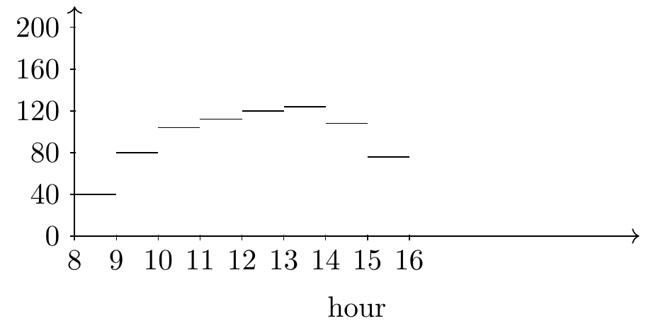
Figure 5.1: A demand profile.
It is also easy to find the service distribution; for ease, we model the service time distribution as exponential with mean \(1.5\) minutes.
For the service objective we prefer to keep the average number of jobs in the system such that \(\E \L \leq 5\).2Other KPIs are also possible to use.
Let us model the situation as an \(M/M/1\) queue with one server that works as fast as \(c\) single servers combined. Solving for \(c\) in the inequality \(\E \L \leq 5\) gives3\(\E \L = \rho/(1-\rho) \implies \rho = \E \L/(\E \L + 1)\) and \(\rho=\lambda \E S /c\).
\begin{equation*} c \geq \frac{\E \L + 1}{\E \L} \lambda \E S = \frac 6 5 \lambda \E S \approx 0.03 \lambda, \end{equation*}where, with the above estimate, \(\E{S}=1.5/60\) hour. It is easy to apply this formula. For instance, we see in the demand profile Fig. 5.1 that \(\lambda= 120\) customers per hour between 12 and 13, hence we need \(c\approx 3.6 = 4\) employees for that period.
With this we can find a formula to convert the demand profile into a load profile to specify the minimal number of servers per hour needed to meet the service objective.
The last step in the planning process is to cover the load profile with service shifts. This is typically not easy since shifts have to satisfy all kinds of restrictions with respect to breaks and durations. Moreover, shifts can also have different costs: evening shifts are typically more expensive per hour.
The usual way to solve such covering problems is by means of an integer programming problem. For instance, suppose only 4 shift plans are available as shown at the right.41. \(++-++\) 2. \(+++-+\) 3. \(++-+++\) 4. \(+++-++\). Shift plans. A \(+\) indicates a working hour and \(-\) a break of an hour.
For the optimization, let \(x_i\) be the number of shifts of type \(i\) and \(c_i\) the cost of this type. Then the problem is to solve \(\min \sum_i c_i x_i\), such that for all hours \(t\) the shifts cover the load, that is, \(\sum_i x_i \1{t \in s_i} \geq 0.03 \lambda_t\). (We write \(t\in s_i\) if hour \(t\) is covered by shift type \(i\).)
TF 1.
Suppose \(\frac{\lambda}{\mu} = 2\). Claim: 3 is the minimum number of servers required to make the system stable.
Solution
Did you actually try? Write your solution down first for comparison.
Show the solution
True.
TF 2.
Claim: It is always better to have a single fast server than multiple slow servers which together have the same rate.
Solution
Did you actually try? Write your solution down first for comparison.
Show the solution
False. This depends on the objective. The service time at a slow server is longer. However, when multiple servers are present, if one server breaks down, service can still continue with the other servers, while when a single fast server fails, everything stops.
TF 3.
A repair/maintenance facility would like to determine how many employees should be working in its tool crib. The service time is exponential, with a mean of 4 minutes, and customers arrive as a Poisson process with a rate of 28 per hour. Claim: With one employee the system is not rate stable.
Solution
Did you actually try? Write your solution down first for comparison.
Show the solution
True.
TF 4.
Consider an \(M/M/c/K\) queue that is not rate stable, but jobs sometimes balk. Claim: \(\lim\limits_{t\to\infty}\mathbb{P}(L(t)=K)=1\).
Solution
Did you actually try? Write your solution down first for comparison.
Show the solution
False. Just after jobs balk, the number of jobs in the system is less than \(K\).
TF 5.
Claim: For the \(M/M/c\) queue, adding a second server always halves the expected waiting time compared to the \(M/M/1\) queue with the same arrival and service rates.
Solution
Did you actually try? Write your solution down first for comparison.
Show the solution
False. Adding a second server reduces the waiting time, but not by exactly half. The reduction depends nonlinearly on \(\rho\) and is typically much more than a factor \(2\).
The next exercises require some modeling skills. Hence, they may be quite hard even though the formulas are simple.
Exercise 6.
In the town hall of the municipality, people can, for example, renew their driver’s license or passport. For ease, assume that there is just one employee and that the arrivals of customers are not planned. Why is it reasonable to model this queueing system as a \(M/M/1\) queue?
Measurements show that \(\E \W = 6\) minutes and \(\lambda=5\) per minute. What are the service rate and utilization? Calculate \(\E{\QQ}\), \(\E \L\).
There should be a sufficient number of seats so that all waiting customers can sit down at least 90 percent of the time. How many seats should there minimally be? What would you advise the municipality?
Hint
\(\E{\QQ}\) follows right away from an application of Little’s law. For the other quantities, we need to find \(\E S\). Use the expression for \(\E\W\) for the queue \(M/M/1\) to solve for \(\rho\). Then, since \(\lambda\) is known, \(\E S\) follows.
Solution
Did you actually try? Write your solution down first for comparison.
Show the solution
As people arrive without making appointments, it is reasonable to say that the inter-arrival times are memoryless. As for the services, the employee deals with many different questions, some are short, some are long. So, we also model service times as exponential.
With Little’s law:
\[ \E\QQ=\lambda\E\W=5\cdot6=30. \] Moreover, \(\E S=\rho/\lambda\), so the waiting-time formula gives \[ 6=\frac{\rho}{1-\rho}\frac{\rho}{5}. \] Solving this quadratic equation yields
\begin{align*} \rho &\approx 0.9687, & \E S &\approx 0.1937\text{ minutes}. \end{align*}Therefore,
\begin{align*} \mu &= 1/\E S\approx5.161\text{ per minute}, & \E J &= \E W+\E S\approx6.1937\text{ minutes}. \end{align*}Thus, \(\E L=\lambda\E J\approx30.9687\).
With \(s\) seats, all waiting customers can sit precisely when \(L\leq s+1\): one customer can be at the employee’s desk. Since \(\P{L\leq k}=1-\rho^{k+1}\), we need \[ 1-\rho^{s+2}\geq0.9. \] The smallest solution is \(s=71\). This very large number confirms that the municipality should hire another employee rather than provide so many seats.
The average queue is huge: hire an extra employee.
Exercise 7.
The smallest barber shop in town works alone and has two chairs for waiting customers. Six jobs arrive per hour, and the barber needs 12 minutes for a haircut. We model this, for ease, as an \(M/M/1/3\) queue. Estimate \(\E{\QQ}\) and the average number of customers served per hour. Then, estimate \(\E{\QQ}\) when the barber hires another location that allows for 3 extra chairs. Quantify the effect on the number of customers served per hour.
Solution
Did you actually try? Write your solution down first for comparison.
Show the solution
This is an \(M/M/1/3\) queue: there is room for 1 customer in service and two in queue.
Write \(K\) for the total system capacity and \(\rho=\lambda/\mu=6/5\). The level-crossing equations give \[ p(n)=\frac{\rho^n}{\sum_{j=0}^{K}\rho^j},\qquad 0\leq n\leq K. \] With two waiting chairs, \(K=3\). Therefore, \[ (p(0),\ldots,p(3))\approx(0.186,0.224,0.268,0.322), \] and \[ \E\QQ=\sum_{n=0}^{3}(n-1)^+p(n)\approx0.912. \] Jobs are accepted, and hence served, at rate \[ \bar\lambda=\lambda(1-p(3))\approx4.069\text{ per hour}. \]
With three extra waiting chairs, \(K=6\). The same calculation gives
\begin{align*} \E\QQ &\approx 2.787, & \bar\lambda &= \lambda(1-p(6))\approx4.613\text{ per hour}. \end{align*}Thus, the extra chairs increase the throughput only modestly and create a longer queue. Since the barber is overloaded, an extra server is more useful.
Exercise 8.
Occasionally there is a pizza stand at the corner of the Verlengde Visserstraat and the Westersingel in Groningen. As people (tend to) behave like sheep, the rate at which people join the queue depends on the actual queue length. When there is nobody waiting, people are somewhat hesitant to order: `When there are no people waiting, most likely the pizzas are not good.’. However, when the queue is long, people prefer to go elsewhere. Measurements show that the number of arrivals per hour is well captured by the array \(\lambda=\qb{10,10,20,20,5}\), where entry \(n\) is the arrival rate when there are \(n\) customers in the system. The pizza oven can contain two pizzas and it takes 2 minutes to bake a pizza. We model the system as an \(M/M/2\) queue.
Calculate the steady-state probabilities and from this the average arrival rate. Then, find \(\E \L\), \(\E{\QQ}\), \(\E \J\) and \(\E{\W}\).
Solution
Did you actually try? Write your solution down first for comparison.
Show the solution
The state-dependent service rates are
\begin{align*} \mu(0) &= 0, & \mu(1) &= 30, & \mu(n) &= 60\quad\text{for }n\geq2. \end{align*}Starting with \(q(0)=1\), the level-crossing recursion \[ q(n+1)=q(n)\frac{\lambda(n)}{\mu(n+1)} \] and normalization give \[ (p(0),\ldots,p(5)) \approx(0.7072,0.2357,0.0393,0.0131,0.0044,0.0004). \] Consequently, \[ \bar\lambda=\sum_{n=0}^{4}\lambda(n)p(n)\approx10.4984, \]
\begin{align*} \E L &= \sum_{n=0}^{5}np(n)\approx0.3729, & \E\QQ &= \sum_{n=0}^{5}(n-2)^+p(n)\approx0.0229. \end{align*}Little’s law then yields \[ \E J=\frac{\E L}{\bar\lambda}\approx0.0355\text{ hours} \approx2.13\text{ minutes}, \] and \[ \E W=\frac{\E\QQ}{\bar\lambda}\approx0.00218\text{ hours} \approx0.13\text{ minutes}. \]
Exercise 9.
Fast food restaurants tend to fry patties before customers arrive. This way, they can serve customers faster, because when a customer arrives while there is still an inventory of prepared patties, the server only has to flip a patty in a bun, while otherwise the customer has to wait for the additional frying time of the patty. Assume the restaurant keeps at most 3 patties on stock. To keep the model simple, assume the restaurant has just one pan to fry a patty and the frying time \(S\sim \Exp{\mu}\) with \(\mu = 15\) per hour. Customers arrive as a Poisson process with rate \(\lambda=12\) per hour. When there is a prepared patty upon arrival, the customer is served immediately, otherwise the customer has to wait for a patty.
Explain how to model this system as an \(M/M/1\) system. Then compute the average number of patties on stock, the average number of people waiting, and the average waiting time of a patty before it ends up in a bun, and the average time a person has to wait for a hamburger.
You should remember this problem. It is of fundamental importance in inventory control and known as an inventory system with backlogging; it is (implicitly) used by nearly any company that keeps inventory.
Hint
Let \(T\) be the number of patties waiting and \(G\) the number of persons waiting. There cannot be a patty and a person waiting at the same time, hence \(T\cdot G = 0\). Take \(L\) as the number of jobs in an \(M/M/1\) queue. If \(L=0\), then there are 3 patties on stock, when \(L=1\) there is one patty less \(T=2, G=0\); when \(L=2\), we have two patties less, so \(T=1, G=0\), when \(L=3\), there are no patties on stock, but also no people waiting, hence \(T=0, G=0\). When \(L=4\), we ran out of patties and one person must be waiting, hence \(T=0, G=1\).
With this reasoning we see a pattern: at all moments in time, \(3=T+L - G\). Now map this system to an \(M/M/1\) queue.
Solution
Did you actually try? Write your solution down first for comparison.
Show the solution
The rv \(L\) behaves like the number of jobs in an \(M/M/1\) queue. If we have \(L\), then with the two properties \(T G = 0\) and \(3 = T +L - G\), we can retrieve (uniquely at all moments in time) the number of patties \(T\) on stock and the number of people waiting \(G\). In inventory terms, \(G\) represents the number of backlogged patties.
With this mapping, the expected number of patties on stock is \(\E T = \sum_{l=0}^3 (3-l)p(l)\). Here \(\rho=\lambda/\mu=0.8\) and \(p(l)=(1-\rho)\rho^l\), so \[ \E T=\sum_{l=0}^{2}(3-l)(1-\rho)\rho^l=1.048. \]
For the expected number of people waiting, use that \(3=T+L-G\) always. Taking expectations gives \[ \E G=\E T+\E L-3 =1.048+\frac{0.8}{1-0.8}-3 =2.048. \]
In steady state, patties are produced and customers arrive at the same average rate \(\lambda\). Little’s law therefore gives \[ \frac{\E T}{\lambda}=\frac{1.048}{12}\text{ hour}\approx5.24\text{ minutes} \] for the average time a patty waits before it ends up in a bun, and \[ \frac{\E G}{\lambda}=\frac{2.048}{12}\text{ hour}\approx10.24\text{ minutes} \] for the average time a customer waits for a hamburger.
What would be the impact of allowing 4 patties maximally?
Exercise 10.
[Continuation of Exercise 9] What would be the impact of allowing four patties on stock?
Hint
How is the invariant \(3 = T + L -G\) affected?
Solution
Did you actually try? Write your solution down first for comparison.
Show the solution
The invariant \(3 = T + L -G\) becomes \(4 = T + L -G\).
The queue itself does not change, so \(\rho=0.8\) and \(p(l)=(1-\rho)\rho^l\) still apply. Hence,
\begin{align*} \E T &= \sum_{l=0}^{3}(4-l)(1-\rho)\rho^l=1.6384, & \E G &= \E T+\E L-4=1.6384. \end{align*}Compared with a maximum of three patties, more patties wait in stock, while fewer customers wait for a hamburger. In particular, the average customer waiting time decreases to \[ \frac{\E G}{\lambda}=\frac{1.6384}{12}\text{ hour}\approx8.19\text{ minutes}. \]
Exercise 11.
[Continuation of Exercise 9] Suppose that the restaurant does not keep patties in stock. What is the expected waiting time for the customer?
Solution
Did you actually try? Write your solution down first for comparison.
Show the solution
The invariant \(3 = T + L -G\) becomes \(0 = T + L -G\). This implies that \(T=0\) and \(L=G\). Hence \(\E G = \E \L=\rho/(1-\rho)=4\), and the expected customer waiting time is \[ \frac{\E G}{\lambda}=\frac{4}{12}\text{ hour}=20\text{ minutes}. \]