3.3 Simulating Waiting Times
3.3 Simulating Waiting Times
Using the recursions of Section 3.1, we can simulate the waiting time of the \(G/G/1\) queue. We use this to analyze how various blocking strategies can prevent long waiting times. In passing we will encounter subtle problems with stochastic dependence and with (plotting) pmfs.
The dynamics of the single-server queue in continuous time is given by the recursions in (3.1.1).
Suppose that the inter-arrival times \(\qb{x_1,\ldots,x_n}\) and service times \(\qb{s_1,\ldots,s_n}\) of one sample path are given. The next algorithm computes the arrival, departure, waiting, and sojourn times of all jobs.
\begin{algorithm}
\caption{Simulation: compute a sample path of a single-server queue.}
\begin{algorithmic}[1]
\State \textbf{Input:} inter-arrival times \(\qb{x_1,\ldots,x_n}\) and service times \(\qb{s_1,\ldots,s_n}\)
\State \textbf{Output:} arrival times \(A\), departure times \(D\), waiting times \(W\), and sojourn times \(J\)
\Procedure{QueueSamplePath}{\(\qb{x_1,\ldots,x_n},\qb{s_1,\ldots,s_n}\)}
    \State \(A_0\gets0\), \(D_0\gets0\)
    \For{\(k=1,\ldots,n\)}
        \State \(A_k\gets A_{k-1}+x_k\)
        \State \(D_k\gets\max\{A_k,D_{k-1}\}+s_k\)
        \State \(J_k\gets D_k-A_k\)
        \State \(W_k\gets J_k-s_k\)
    \EndFor
    \Return \(A,D,W,J\)
\EndProcedure
\end{algorithmic}

\end{algorithm}
Once the sample path is available, its average waiting and sojourn times and its time-average number of jobs are
\begin{equation*} \overline W=\frac{\pr{Sum}\rb{\qb{W_1,\ldots,W_n}}}{n}, \qquad \overline J=\frac{\pr{Sum}\rb{\qb{J_1,\ldots,J_n}}}{n}, \qquad \bar L=\frac{\pr{Sum}\rb{\qb{J_1,\ldots,J_n}}}{D_n}. \end{equation*}For a threshold \(T\), the fraction of jobs whose waiting time is at least \(T\) is
\begin{equation*} q_T = \frac{\pr{Sum}\rb{\qb{\1{W_k\geq T}:k=1,\ldots,n}}}{n}. \end{equation*}For example, take independent exponential inter-arrival and service times with rates \(\lambda=1\) and \(\mu=1.1\), respectively. For one sample path of \(10\,000\) jobs, we obtain \(\overline J=10.11\), \(\overline W=9.20\), and \(\bar L=10.167\). The maximum waiting time is \(52.12\), and \(q_5=0.59\).
Blocking jobs can be a remarkably effective strategy to prevent long and variable waiting times. One rule, known as complete acceptance, accepts job \(k\) when \(\W_k\leq T\) and otherwise blocks it; see Alg. 3.3.2. The algorithm records this decision with the indicator \(I_k\), which is \(1\) for an accepted job and \(0\) for a rejected job. Hence, if job \(k-1\) is accepted, \(I_{k-1}s_{k-1}=s_{k-1}\) contributes to \(\W_k\); if it is rejected, \(I_{k-1}s_{k-1}=0\), so it adds no work to the system. In this way, blocking is implemented without modifying the original service times.
\begin{algorithm}
\caption{Apply complete acceptance with waiting-time threshold \(T\).}
\begin{algorithmic}[1]
\State \textbf{Input:} inter-arrival times \(\qb{x_1,\ldots,x_n}\), service times \(\qb{s_1,\ldots,s_n}\), and threshold \(T\)
\State \textbf{Output:} waiting times \(W\) and acceptance decisions \(I\)
\Procedure{CompleteAcceptance}{\(\qb{x_1,\ldots,x_n},\qb{s_1,\ldots,s_n},T\)}
    \State \(W_1\gets0\), \(I_1\gets1\) \Comment{The system starts empty}
    \For{\(k=2,\ldots,n\)}
        \State \(W_k\gets[W_{k-1}+I_{k-1}s_{k-1}-x_k]^+\)
        \State \(I_k\gets\1{W_k\leq T}\)
    \EndFor
    \Return \(W,I\)
\EndProcedure
\end{algorithmic}

\end{algorithm}
The fraction of accepted jobs and the average waiting time of accepted jobs are, respectively,
\begin{equation*} a=\frac{\pr{Sum}\rb{\qb{I_1,\ldots,I_n}}}{n}, \qquad \overline W_{\mathrm{accepted}} = \frac{\pr{Sum}\rb{\qb{I_kW_k:k=1,\ldots,n}}} {\pr{Sum}\rb{\qb{I_1,\ldots,I_n}}}. \end{equation*}nFor the sample path above, \(a=0.90\), the average waiting time over all jobs is \(2.23\), and \(\overline W_{\mathrm{accepted}}=1.83\). Moreover, \(8994\) of the \(10\,000\) jobs are accepted, and the maximum waiting time of an accepted job is \(5.00\). Thus, about \(90\%\) of the jobs are accepted, while the average waiting time drops by a factor of about four and the maximum by more than a factor of ten.
There are other interesting rules to block jobs. A second rule, complete rejection, accepts only if \(\J_k \leq T\); see Alg. 3.3.3. Here, \(J_k=W_k+s_k\) is the sojourn time job \(k\) would have if it were accepted. Thus, unlike complete acceptance, complete rejection also takes the service time of the arriving job into account. As before, \(I_{k-1}s_{k-1}\) ensures that a rejected job adds no work to \(W_k\).
\begin{algorithm}
\caption{Apply complete rejection with sojourn-time threshold \(T\).}
\begin{algorithmic}[1]
\State \textbf{Input:} inter-arrival times \(\qb{x_1,\ldots,x_n}\), service times \(\qb{s_1,\ldots,s_n}\), and threshold \(T\)
\State \textbf{Output:} waiting times \(W\), candidate sojourn times \(J\), and acceptance decisions \(I\)
\Procedure{CompleteRejection}{\(\qb{x_1,\ldots,x_n},\qb{s_1,\ldots,s_n},T\)}
    \State \(W_1\gets0\), \(J_1\gets s_1\), \(I_1\gets\1{J_1\leq T}\) \Comment{The system starts empty}
    \For{\(k=2,\ldots,n\)}
        \State \(W_k\gets[W_{k-1}+I_{k-1}s_{k-1}-x_k]^+\)
        \State \(J_k\gets W_k+s_k\)
        \State \(I_k\gets\1{J_k\leq T}\)
    \EndFor
    \Return \(W,J,I\)
\EndProcedure
\end{algorithmic}

\end{algorithm}
For the arrival and service times above, the average waiting time over all jobs is \(1.21\), and the average service time of accepted jobs is \(0.75\). The largest service time among all jobs is \(9.25\), whereas the largest service time among accepted jobs is \(4.92\). Perhaps surprisingly, for the same arrival and service times, complete rejection accepts \(0.97\) of the jobs, compared with \(0.90\) under complete acceptance. Although complete rejection uses a stricter admission rule, it rejects a job before that job adds work1In particular, all jobs \(\geq T\) are rejected. to the system whenever \(W_k+s_k>T\). This reduces the waiting times of later jobs, so more of them can be accepted.
A third rule, partial acceptance, admits as much of each job’s service requirement as possible without making its sojourn time exceed \(T\); see Alg. 3.3.4. Thus, after job \(k\) has waited \(W_k\), at most \(T-W_k\) units of its required service time \(s_k\) can be accepted. If \(B_k\) denotes the accepted part, then
\begin{align*} B_k &= \min\{T-W_k,s_k\}, & J_k &= W_k+B_k. \end{align*}
\begin{algorithm}
\caption{Apply partial acceptance with sojourn-time threshold \(T\).}
\begin{algorithmic}[1]
\State \textbf{Input:} inter-arrival times \(\qb{x_1,\ldots,x_n}\), service times \(\qb{s_1,\ldots,s_n}\), and threshold \(T\)
\State \textbf{Output:} waiting times \(W\), accepted service times \(B\), and sojourn times \(J\)
\Procedure{PartialAcceptance}{\(\qb{x_1,\ldots,x_n},\qb{s_1,\ldots,s_n},T\)}
    \State \(W_1\gets0\), \(B_1\gets\min\{T,s_1\}\), \(J_1\gets B_1\) \Comment{The system starts empty}
    \For{\(k=2,\ldots,n\)}
        \State \(W_k\gets[W_{k-1}+B_{k-1}-x_k]^+\)
        \State \(B_k\gets\min\{T-W_k,s_k\}\)
        \State \(J_k\gets W_k+B_k\)
    \EndFor
    \Return \(W,B,J\)
\EndProcedure
\end{algorithmic}

\end{algorithm}
For the arrival and service times above, the average waiting time is \(1.58\), the average sojourn time is \(2.36\), and the average accepted service time is \(0.78\). The largest accepted service time is \(5.00\), as required.
We next show how to obtain the \emph{distribution} of the waiting time and departure time of job \(k=30\).2Job \(k=30\) is chosen arbitrarily. We use both the probabilistic arithmetic of Section 1.4 and simulation.
The inter-arrival and service distributions are as follows. We choose \(\E S > \E X\) to get more widely spread values in the figures.
\begin{equation*} p_X(3)=p_X(4)=p_X(5)=\frac13, \qquad p_S(4)=p_S(5)=p_S(7)=\frac13, \tag{3.3.1} \end{equation*}and both pmfs are zero elsewhere. Thus, \(\E X=4\) and \(\E S=16/3\approx5.33\).
Since the system starts empty, \(\P{\W_1=0}=1\). The procedure in Alg. 3.3.5 repeatedly applies the probabilistic-arithmetic procedures from Section 1.4 to Lindley’s recursion. Each iteration uses fresh independent copies of \(X\) and \(S\). This is valid because \(W_{k-1}\) is independent of \(S_{k-1}\) and \(X_k\).
\begin{algorithm}
\caption{Exact calculation: compute the pmf of the waiting time of job \(n\).}
\begin{algorithmic}[1]
\State \textbf{Input:} inter-arrival-time pmf \(p_X\), service-time pmf \(p_S\), and job number \(n\)
\State \textbf{Output:} waiting-time pmf \(p_W\) of \(W_n\)
\Procedure{WaitingTimePMF}{\(p_X,p_S,n\)}
    \State \(p_W\gets\pr{Constant}\rb{0}\) \Comment{The system starts empty}
    \For{\(k=2,\ldots,n\)}
        \State \(p_W\gets\pr{Add}\rb{p_W,p_S}\)
        \State \(p_W\gets\pr{Subtract}\rb{p_W,p_X}\)
        \State \(p_W\gets\pr{PositivePart}\rb{p_W}\)
    \EndFor
    \Return \(p_W\)
\EndProcedure
\end{algorithmic}

\end{algorithm}
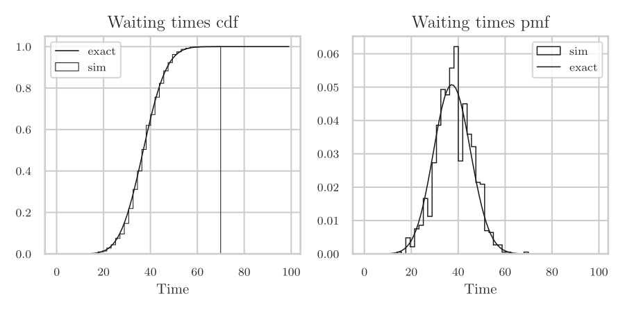
We compare the distribution obtained by probabilistic arithmetic with an estimate based on simulation. The mean and standard deviation of the waiting time obtained by probabilistic arithmetic are \(37.51\) and \(7.82\), respectively. The simulation estimates are \(37.36\) and \(7.61\), which agree well. Fig. 3.1 compares the theoretical and simulated cdfs and pmfs of \(\W_{30}\).
Let us now compare \(D_{30}\) computed with probabilistic arithmetic with the simulated departure time, which we denote by \(\hat D_{30}\). Recall that \(D_{30}=A_{30}+W_{30}+S_{30}\). Thus, to compute \(D_{30}\) with probabilistic arithmetic, we need the pmfs of \(A_{30}\), \(W_{30}\), and \(S_{30}\). Since \(A_{30}=\sum_{k=1}^{30}X_k\), we obtain its pmf as \(p_{A_{30}}\gets\pr{Convolution}\rb{p_X,30}\). The procedure in Alg. 3.3.5 provides the pmf of \(W_{30}\). Finally, \(S_{30}\) has the pmf \(p_S\) specified in (3.3.1). Combining these three pmfs as if the random variables were independent gives a mean of \(158.84\) and a standard deviation of \(9.06\). In contrast, \(\hat D_{30}\) has simulated mean \(158.74\) and standard deviation \(6.45\). The means are close, but the standard deviations differ noticeably. The probabilistic-arithmetic result is wrong.
The reason is that \(A_k\) and \(\W_k\) are negatively correlated. Recall that \(A_k = A_{k-1}+X_k\) and \(\W_k = [\W_{k-1} + S_{k-1} - X_k]^+\). If \(X_k\) is very large, \(A_k\) is large, but \(\W_k\) is zero (or small), and then \(D_k \approx A_{k} + S_{k}\) . In probabilistic arithmetic, addition of two rvs is only allowed when they are independent.3Handling such dependencies requires the modeling of the joint distribution of rvs. The Python package lea supports this. Treating \(A_k+W_k+S_k\) as the sum of three independent rvs violates this assumption. But why then is the recursion \(\W_k = [\W_{k-1} + S_{k-1} - X_k]^{+}\) correct? This is because \(\W_{k-1}\) \emph{is} independent of \(S_{k-1}\) and \(X_{k}\).
Stochastic dependence is easily overlooked. To avoid making mistakes, check analytical results with simulation. If the results disagree, there is probably an error4Often not just one error! somewhere.
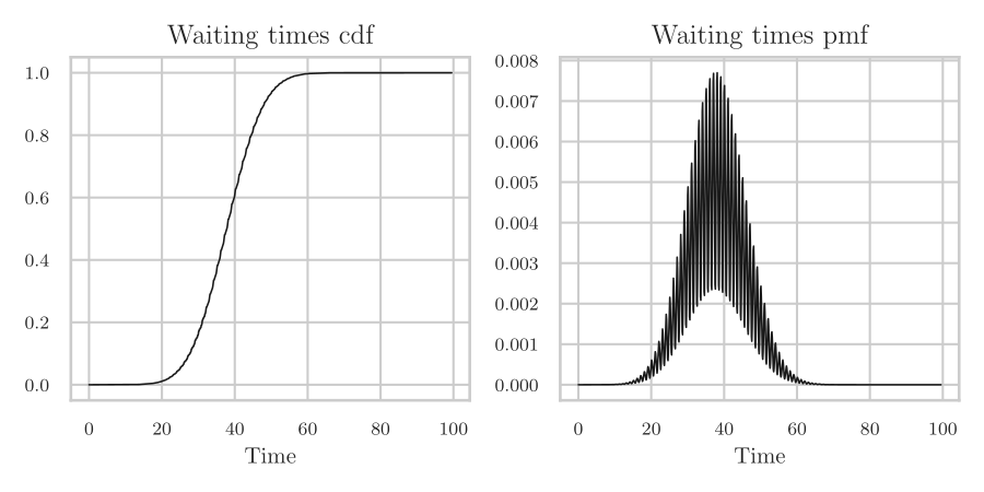
In general, the cdf behaves more regularly than the pmf, even though the pmf seems easier to interpret. To show this, modify the support of \(X\) to \(\{3, 4.1, 5\}\), keep all else the same, and simulate. The resulting pmf in 2 differs markedly from that in 1!
X = RV({4.1: 1 / 3, 5: 1 / 3, 3: 1 / 3})
S = RV({4: 1 / 3, 5: 1 / 3, 7: 1 / 3})

horizon = 30
A = RV({0: 1})  # arrival time
W = RV({0: 1})  # waiting time
for i in range(1, horizon):
    A += X
    W = (W + S - X).map(Plus)

fig, (ax1, ax2) = plt.subplots(nrows=1, ncols=2, figsize=(6, 3))
ax1.set_title("Waiting times cdf")
ax1.set_xlabel("Time")
ax1.plot(
    W.support(), [W.cdf(k) for k in W.support()], c='k', lw=0.75, label="exact"
)
ax2.set_title("Waiting times pmf")
ax2.set_xlabel("Time")
ax2.plot(
    W.support(), [W.pmf(k) for k in W.support()], c='k', lw=0.75, label="exact"
)

fig.tight_layout()
fig.savefig("../figures/waiting_time_distribution_pmf_4.1.pdf")
We finish this section with the multi-server queue of (3.1.9). Let \(w(i)\) be the time until server \(i\) becomes available. During an inter-arrival time \(x_k\), every component of \(w\) decreases by \(x_k\), but cannot become negative. Job \(k\) then selects a server with the smallest workload. If server \(i_k\) has rate \(\mu(i_k)\), its service takes \(s_k/\mu(i_k)\) time.
\begin{algorithm}
\caption{Compute a sample path of a multi-server queue.}
\begin{algorithmic}[1]
\State \textbf{Input:} inter-arrival times \(\qb{x_1,\ldots,x_n}\), work requirements \(\qb{s_1,\ldots,s_n}\), and server rates \(\qb{\mu(1),\ldots,\mu(c)}\)
\State \textbf{Output:} selected servers \(i\), arrival times \(A\), departure times \(D\), waiting times \(W\), and sojourn times \(J\)
\Procedure{MultiServerQueue}{\(x,s,\mu\)}
    \State \(A_0\gets0\), \(w\gets\qb{0,\ldots,0}\)
    \For{\(k=1,\ldots,n\)}
        \State \(A_k\gets A_{k-1}+x_k\)
        \State \(w\gets[w-x_k\mathbf{1}]^+\)
        \State \(i_k\gets\argmin_{j\in\{1,\ldots,c\}}w(j)\)
        \State \(W_k\gets w(i_k)\)
        \State \(J_k\gets W_k+s_k/\mu(i_k)\)
        \State \(D_k\gets A_k+J_k\)
        \State \(w(i_k)\gets w(i_k)+s_k/\mu(i_k)\)
    \EndFor
    \Return \(i,A,D,W,J\)
\EndProcedure
\end{algorithmic}

\end{algorithm}
The algorithm allows the server rates to differ. Setting \(\mu(i)=1\) for every server gives the special case used in the previous numerical example.
TF 1.
The list \(D=\qb{D_0,D_1,\ldots,D_n}\) contains the departure times computed by a queue simulation. Here \(D_0=0\) is used only for initialization and does not correspond to a job.
\begin{algorithm}
\begin{algorithmic}[1]
\State \(m\gets\pr{Sum}\rb{D}/(n+1)\)
\end{algorithmic}

\end{algorithm}
Claim: \(m\) is the mean departure time of the \(n\) simulated jobs.
Solution
Did you actually try? Write your solution down first for comparison.
Show the solution
False. The initialization \(D_0\) should not be included. The mean departure time is \[ \frac{\pr{Sum}\rb{\qb{D_1,\ldots,D_n}}}{n}. \]
TF 2.
Consider a continuous-time queue with inter-arrival times \(\{X_k\}\), service times \(\{S_k\}\), waiting times \(\{\W_k\}\), and sojourn times \(\{\J_k\}\). Claim: we can compute the waiting times and sojourn times using the recursion:
\begin{align*} \W_k &= [\J_{k-1} - X_k]^+, & \J_k &= \W_k + S_k. \end{align*}Solution
Did you actually try? Write your solution down first for comparison.
Show the solution
True.
TF 3.
Let \(p_X\) and \(p_S\) be the pmf maps of the inter-arrival and service times. Consider the following algorithm.
\begin{algorithm}
\begin{algorithmic}[1]
\State \(p_A\gets\pr{Constant}\rb{0}\)
\State \(p_D\gets\pr{Constant}\rb{0}\)
\For{\(k=1,\ldots,n\)}
    \State \(p_A\gets\pr{Add}\rb{p_A,p_X}\)
    \State \(p_D\gets\pr{Maximum}\rb{p_D,p_A}\)
    \State \(p_D\gets\pr{Add}\rb{p_D,p_S}\)
\EndFor
\Return \(p_D\)
\end{algorithmic}

\end{algorithm}
Claim: this algorithm correctly computes the pmf of \(D_n\).
Solution
Did you actually try? Write your solution down first for comparison.
Show the solution
False. The call to \(\pr{Maximum}\) incorrectly treats \(A_k\) and \(D_{k-1}\) as independent.
TF 4.
In a \(G/G/c\) queue, job \(k\) sees the workload \(w(j)\) and service rate \(\mu(j)\) of each server \(j\). Consider the following selection rule.
\begin{algorithm}
\begin{algorithmic}[1]
\State \(i_k\gets\argmin_{j\in\{1,\ldots,c\}}w(j)\)
\State \(W_k\gets w(i_k)\)
\State \(J_k\gets W_k+s_k/\mu(i_k)\)
\end{algorithmic}

\end{algorithm}
Claim: this rule selects the server that gives job \(k\) the smallest sojourn time.
Solution
Did you actually try? Write your solution down first for comparison.
Show the solution
False. It selects the server with the smallest waiting time. When service rates differ, the smallest sojourn time is obtained by selecting \[ \argmin_{j\in\{1,\ldots,c\}}\{w(j)+s_k/\mu(j)\}. \]
TF 5.
Claim: In a \(G/G/c\) queue simulation, the waiting time of job \(k\) can be computed as \(\W_k = [\W_{k-1} + S_{k-1} - X_k]^+\).
Solution
Did you actually try? Write your solution down first for comparison.
Show the solution
False. This recursion is only valid for the \(G/G/1\) queue with a single server. For \(c > 1\) servers, we must track the workload at each server and assign the job to the server that becomes free earliest.