4 Trees, Bags, and Random Forests
On this page
Instead of paying for a route planner such as Komoot,1A mobile app for
navigation and route planning,
Wikipedia: Komoot. why not try to
build our own? OpenStreetMap (OSM) offers map data. From this we can get edges and
features of edges such as highway classification (path, track, primary
road, \ldots), surface (sand, asphalt, gravel, \ldots), and access
restrictions. Binary features indicate whether an edge lies in a protected area
or crosses a bridge or tunnel. We also compute spatial features
ourselves, for instance the distance to the nearest forest, water, or motorway.
Then we need labeled edges that tell us whether an edge is good (0) or bad (1).
We label edges in published walks such as the Pieterpad as good. We call an edge bad if it lies in an industrial zone or
next to a motorway. With these labeled edges, we can train a classifier that can
score new, unlabeled edges. We convert these scores into edge costs, find a
minimum-cost path from a point \(A\) where we want to start our walk to the
finish \(B\), and plot it on a map. In this chapter we show how to set up a
classifier for our map, which contains about \(10^7\) edges.
A binary decision tree can score an edge by asking yes/no questions about its features: is the highway type a major road? is the distance to the nearest forest below 100 m? is the surface paved? Each answer selects a branch. At a leaf, the tree returns the fraction of training edges in that leaf labeled bad. For our walking app, this fraction lies in \([0, 1]\) by construction.
In slightly more abstract terms,2Wikipedia: Decision tree learning. a tree maps a feature vector \(x\) to a prediction \(\hat a=T(x)\). Each internal node stores a split rule and two child nodes; each leaf stores a prediction.
A single tree is easy to interpret, but deep trees can be unstable: small changes in the training data can change their splits and predictions. This is high variance. Bagging, random forests, and boosting are useful ensemble methods that combine trees to reduce this instability.
4.1 Decision trees
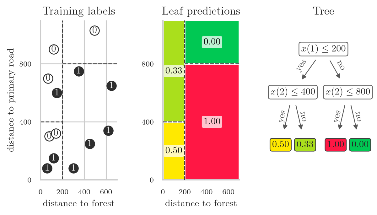
Consider two features: distance to a forest, \(x(1)\), and distance to a primary road, \(x(2)\), both in meters.3For the real app, we use many more features. The left panel in Fig. 4.1 shows a few edges that have been labeled: \(y=0\) means that the edge is a good edge, and \(y=1\) means that it is a bad edge. If we use \(200\) to split on the distance to forest, and then use \(400\) or \(800\) for the primary road on the left or right branch respectively, the splits place 4 samples in the lower-left rectangle. Their mean label is \(0.5\), which becomes the leaf prediction. The tree predicts an estimated probability \(0.5\) for an edge routed to this rectangle. For the new edge \(x_{\mathrm{new}}=(60,700)\), the tree follows the left branch and then the right branch, reaching the leaf with prediction \(0.33\). The right panel shows this traversal.
Fitting a tree means choosing its splits and leaf predictions to minimize training risk. A leaf gives a constant prediction \(c\) to every sample that reaches it, so the quantities we need are exactly those of Chapter 3: the empirical risk \(\hat R_{\Sset}(c)\) of using \(c\) throughout a list \(\Sset\) of samples, the best such constant \(\hat c(\Sset)\), and the risk \(\hat R_{\Sset}(\hat c(\Sset))\) that it attains. For short, write
\begin{align*} \hat R(\Sset) = \hat R_{\Sset}(\hat c(\Sset)). \end{align*}For regression, these are given by (3.2.3), while for classification we use .
The leaves of a fitted tree form a partition \(\Pset_{\Tset}(T) = \set{\Tset_1, \ldots, \Tset_m}\) of the training set \(\Tset\) such that \(\Tset_{t}\) is the list of samples belonging to a leaf \(t\). The training risk of \(T\) is therefore4Recall, on a leaf \(\hat c(\Tset_{t})\) is constant.
\begin{align*} \hat R_{\Tset}(T) = \frac{1}{|\Tset|} \sum_{t=1}^{m} \sum_{(x,y)\in \Tset_{t}} \lscr(r(y), \hat c(\Tset_{t})) = \frac{1}{|\Tset|} \sum_{t=1}^{m} |\Tset_{t}|\, \hat R(\Tset_{t}). \tag{4.1.1} \end{align*}The training goal can now be stated as an optimization problem5The summation runs over all leaves \(\Sset\) of the tree \(T\) that form the partition of \(\Tset\).
\begin{align*} \min_{T\in \Fset} \sum_{\Sset\in \Pset_{\Tset}(T)} \frac{|\Sset|}{|\Tset|}\, \hat R(\Sset), \tag{4.1.2} \end{align*}where the model class \(\Fset\) is the set of all trees of a given maximal depth.
In general the best tree by exhaustive search is impossible because the number of candidate trees grows rapidly with depth. Let us estimate that growth.
For a binary tree we use a feature coordinate to split the \(n\) samples into a left set with \(l\) elements and a right set with \(n-l\) elements. Assuming distinct feature values, the number of candidate splits at this node is \((n-1)p\).6We can use each of the \(p\) features to split, and then split between any of the \(n\) samples. Assume the tree has depth at most \(h\).7That is, the number of decisions until reaching a leaf node. Then the number of trees \(N_h(n)\) when the depth is \(h\) and the number of samples is \(n\) satisfies the recursion
\begin{align*} N_h(n) &= p \sum_{l=1}^{n-1} N_{h-1}(l)\,N_{h-1}(n-l), & N_{0}(n) &= 1; \end{align*}when \(h=0\) we stop splitting so there is just one tree left. Suppose \(N_h(n)\sim n^{u_h}p^{v_h}\). Matching the exponents of \(p\) in the above master equation gives
\begin{align*} v_{h} &= 1 + 2 v_{h-1}, & v_{0} &= 0, &\implies v_{h} = 2^{h} -1. \end{align*}For \(u_h\), we should solve
\begin{align*} n^{u_{h}} = \sum_{l=1}^{n-1} l^{u_{h-1}} (n-l)^{u_{h-1}}. \end{align*}Approximating the sum by an integral,
\begin{align*} \sum_{l=1}^{n-1} l^{u} (n-l)^{u}= n^{2u}\sum_{l=1}^{n-1} \rb{\frac{l}{n}}^{u} \rb{1-\frac{l}{n}}^{u} \simeq n^{2u+1} \int_{0}^{1} x^{u}(1-x)^{u} \d x. \end{align*}The (beta) integral does not depend on \(n\). So, again matching exponents in the master equation gives
\begin{align*} u_{h} &= 1 + 2 u_{h-1}, & u_{0} &= 0, &\implies u_{h} = 2^{h} -1. \end{align*}Therefore, the rough growth estimate for the number of trees with at most \(h\) levels of splits is
\begin{align*} N_{h}(n) \sim (n\,p)^{2^{h}-1}. \end{align*}For our case, \(n\approx 10^5\), \(p=30\), and \(h=5\), this is about \(10^{200}\).
Greedy splitting is the customary way around the search over all possible trees in (4.1.2). Suppose the current subtree is to be fitted on \(\Tset\). Then we compare two options: make the current node a leaf, or split \(\Tset\) into a left part \(\Lset\) and a right part \(\Rset\) and assume that each part becomes a leaf. The risk for the first option is \(\hat R(\Tset)\), that of the second is
\begin{align*} \frac{|\Lset|}{|\Tset|}\, \hat R(\Lset) + \frac{|\Rset|}{|\Tset|}\, \hat R(\Rset). \tag{4.1.3} \end{align*}If we can split \(\Tset\) such that the risk of the second option is smaller than that of the first, we should split and fit left and right subtrees on their respective parts. By recursion, the risk of the left branch is \(\hat R(\Lset)\), or smaller if it is better to split \(\Lset\) too. Since the argument also holds for \(\Rset\), we obtain \(\hat R_{\Tset}(T) \leq \hat R(\Tset)\).
The task is therefore to find the split that minimizes the risk for the second option. For each feature \(j\), try thresholds at its observed values. A threshold \(\theta\) sends \(z\) left when \(z(j)\leq\theta\), and right otherwise. Keep the split with the lowest weighted leaf risk, provided it improves on leaving the node unsplit. If none does, return \cn{Nil}. The threshold can instead be placed at a midpoint between consecutive distinct feature values.8This gives the same partition of the training samples.
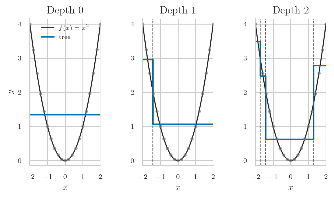
The \cl{Tree} class is implemented in Alg. 4.1.1. The constructor takes a maximum depth and a minimum split size \(\var{min\_elements}\).9These are the tree’s hyperparameters. A node becomes a leaf when its remaining depth is zero or it contains fewer than \(\var{min\_elements}\) samples. Each child receives one less unit of remaining depth. This minimum split size does not prevent a split from producing a singleton leaf. In Fig. 4.1, the initial tree has depth 2, and the leaf node for the lower-left rectangle has depth 0. The effect of the depth parameter is illustrated in Fig. 4.2, where regression trees of depth 0, 1, and 2 are fitted to the function \(f(x)=x^{2}\) on \([-2,2]\).
\begin{algorithm}
\caption{A binary tree class.}
\begin{algorithmic}
\State \textbf{Input:} the maximum depth and the minimum number of samples required to split a node.
\State \textbf{Output:} a tree with fit and predict methods.
\State \textbf{class } $\cl{Tree}(\var{depth}, \var{min\_elements})$
\State $\quad$ \textbf{instance variables:}
\State $\quad\quad \var{left\_tree} \gets \cn{Nil}$
\State $\quad\quad \var{right\_tree} \gets \cn{Nil}$
\State $\quad\quad \var{leaf?} \gets \cn{False}$ \Comment{Is this node a leaf?}
\State $\quad\quad \var{prediction} \gets \cn{Nil}$ \Comment{The prediction when the node is a leaf.}
\State $\quad$ \textbf{methods:}
\State $\quad\quad \pr{Predict}(x)$ \Comment{Return the prediction for the feature vector $x$.}
\State $\quad\quad \pr{Fit}(\Tset)$ \Comment{Fit the tree on a training set $\Tset$.}
\State $\quad\quad \pr{ChooseBranch}(x) \gets \cn{Nil}$ \Comment{Is $x$ in the left or right subtree?}
\end{algorithmic}

\end{algorithm}
Alg. 4.1.2 shows how to set up and use a \cl{Tree} for the example in Fig. 4.1. As in Chapter 3, the training data form a list \(\Tset\) of observations \((x,y)\). Here \(x\) is the feature vector of an edge and \(y\) is its observed label. Once fitted, the tree can return a numerical prediction for a feature vector \(x\) by asking a short sequence of questions about each feature coordinate \(x(j)\).
\begin{algorithm}
\caption{Fit a tree on the training data \Tset of Fig. 4.1, then compute a prediction.}
\begin{algorithmic}
\State $\var{tree} \gets \pr{Tree}(\var{depth} = 2, \var{min\_elements} = 5)$
\State $\var{tree}.\pr{Fit}(\Tset)$ \Comment{Fit the tree on the training set.}
\State $\var{x} \gets [60,700]$
\State $\var{prediction} \gets \var{tree}.\pr{Predict}(\var{x})$  \Comment{Returns the prediction 0.33.}
\end{algorithmic}

\end{algorithm}
The function \pr{Tree.Predict} returns \(\hat a = T(x)\) for a feature vector \(x\), see Alg. 4.1.3. If the current node is a leaf, i.e., when the member variable \var{leaf?} is \cn{True},10Read \var{leaf?} like a question: is this a leaf? More generally, any function or variable with a question mark should be read like “Is this …?”. the method returns the member variable \var{prediction}.11\var{leaf?} and \var{prediction} are set by \pr{Tree.Fit}. The leaf node in Fig. 4.1 corresponding to the lower-left rectangle has prediction \(0.5\). If the current node is not a leaf, the function \pr{ChooseBranch} delegates the prediction to the left or right subtree.12Note, each tree has its own private \pr{ChooseBranch} function.
\begin{algorithm}
\caption{Predict for a feature vector \(x\) using the fitted tree.}
\begin{algorithmic}
\State \textbf{Input:} a feature vector $x$
\State \textbf{Output:} a prediction
\Procedure{Tree.Predict}{$x$}
    \If{$\var{leaf?}$}
        \Return $\var{prediction}$
    \EndIf
    \If{$\pr{ChooseBranch}(x) = \cn{Left}$}
        \Return $\var{left\_tree}.\pr{Predict}(x)$
    \EndIf
    \Return $\var{right\_tree}.\pr{Predict}(x)$
\EndProcedure
\end{algorithmic}

\end{algorithm}
Alg. 4.1.4 searches for the rule that results in the best split into a left and a right part. It first computes the risk if this node would become a leaf. We only split if this risk can be improved. Then we loop over all features and samples in \(\Tset\) to find the split that improves the best rule found so far. The most interesting function is \pr{ChooseBranch}. This uses an anonymous function (\(\lambda\)) that takes an argument and returns a value. Here, we assign to \pr{ChooseBranch} a function that takes a feature vector as argument, and says whether that falls to the left or the right of the threshold \(\theta\).
Here the computation of the threshold is a bit naive. A better implementation takes the threshold halfway between two successive feature values. We skip this complication here.
\begin{algorithm}
\caption{Find the best split rule for a training set \(\Tset\).}
\begin{algorithmic}[1]
\State \textbf{Input:} a non-empty training set $\Tset$.
\State \textbf{Output:} a split rule, or $\cn{Nil}$ if no split into two non-empty parts lowers the training risk
\Procedure{BestSplitRule}{$\Tset$}
    \State $\var{min\_risk} \gets \hat R(\Tset)$ \Comment{Risk if the node becomes a leaf.}
    \State $\var{best\_rule} \gets \cn{Nil}$
    \For{$1\leq j \leq p$} \Comment{Loop over the feature coordinates}
        \For{$(x, y) \in \Tset$} \Comment{Loop over the training samples}
            \State $\theta \gets x(j)$  \Comment{Value of feature coordinate $j$ of this sample}
            \State $\pr{ChooseBranch} \gets \lambda: z \mapsto \cn{Left} \text{ if } z(j) \leq \theta \text{ else } \cn{Right}$
            \State $\Lset \gets \qb{(u, v) \in \Tset : \pr{ChooseBranch}(u) = \cn{Left}}$
            \State $\Rset \gets \qb{(u, v) \in \Tset : \pr{ChooseBranch}(u) = \cn{Right}}$
            \If{$|\Lset| > 0 \text{ and } |\Rset| > 0$}
                \State $\var{risk} \gets \frac{|\Lset|}{|\Tset|}\,\hat R(\Lset) + \frac{|\Rset|}{|\Tset|}\,\hat R(\Rset)$
                \If{$\var{risk} < \var{min\_risk}$}
                    \State $\var{min\_risk} \gets \var{risk}$
                    \State $\var{best\_rule} \gets \pr{ChooseBranch}$
                \EndIf
    \EndIf
        \EndFor
    \EndFor
    \Return $\var{best\_rule}$
\EndProcedure
\end{algorithmic}

\end{algorithm}
This implementation takes \(O(n^2p)\) time: it tries \(np\) thresholds and scans all \(n\) samples for each.13This implementation is horribly inefficient for large data sets: with \(n=10^5\) and \(p=30\), the work is of order \(3\cdot10^{11}\) operations at the root alone. For squared loss, sorting each feature and maintaining running sums of the labels and their squares reduces the split search to \(O(pn\log n)\) time.
\pr{Tree.Fit} uses recursion to fit the tree, see Alg. 4.1.5.14In this pseudocode, \pr{Fit} is called once on a newly constructed object. If a stopping condition holds, Fit stores a leaf prediction. Otherwise, it computes the best split once. If no split lowers the risk, the node also becomes a leaf; otherwise, Fit uses the selected rule to fit each child on the samples sent to it. Each child receives one less unit of remaining depth, so a stopping condition is eventually reached. \pr{SetPrediction}(\Tset) returns the sample mean \(\hat c = \hat y = \frac{1}{|\Tset|}\sum_{(x,y)\in\Tset}y\) for regression, and the class frequencies \(\hat c_{k} = |\qb{(x,y)\in\Tset:y=k}|/|\Tset|\) for classification.
\begin{algorithm}
\caption{Fit a tree recursively to a training set \(\Tset\).}
\begin{algorithmic}[1]
\State \textbf{Input:} a non-empty training set $\Tset$.
\State \textbf{Output:} none
\Procedure{Tree.Fit}{$\Tset$}
    \If{$\pr{StopSplitting?}(\Tset, \var{depth}, \var{min\_elements})$}
        \State $\var{leaf?} \gets \cn{True}$
    \Else
        \State $\pr{ChooseBranch} \gets \pr{BestSplitRule}(\Tset)$
        \If{$\pr{ChooseBranch} = \cn{Nil}$}
            \State $\var{leaf?} \gets \cn{True}$
        \EndIf
    \EndIf
    \If{$\var{leaf?}$}
        \State $\var{prediction} \gets \pr{SetPrediction}(\Tset)$
        \Return
    \EndIf
    \State $\var{left\_tree} \gets \pr{Tree}(\var{depth} - 1, \var{min\_elements})$
    \State $\var{left\_tree}.\pr{Fit}(\qb{(x,y) \in \Tset : \pr{ChooseBranch}(x) = \cn{Left}})$
    \State $\var{right\_tree} \gets \pr{Tree}(\var{depth} - 1, \var{min\_elements})$
    \State $\var{right\_tree}.\pr{Fit}(\qb{(x,y) \in \Tset : \pr{ChooseBranch}(x) = \cn{Right}})$
\EndProcedure
\end{algorithmic}

\end{algorithm}
\pr{StopSplitting?}, see Alg. 4.1.6, checks whether the depth or sample size requires the current node to become a leaf. When \(\var{depth}=0\) or the training set becomes too small, no split is attempted. Otherwise, \pr{Tree.Fit} calls \pr{BestSplitRule} once and checks whether it returns \cn{Nil}. If so, the node also becomes a leaf.
\begin{algorithm}
\caption{Check whether depth or sample size requires the node to become a leaf.}
\begin{algorithmic}
\State \textbf{Input:} a non-empty training set $\Tset$, a depth, and a minimal split size.
\State \textbf{Output:} a Boolean.
\Procedure{StopSplitting?}{$\Tset, \var{depth}, \var{min\_elements}$}
    \If{$\var{depth} = 0$}
        \Return $\cn{True}$
    \EndIf
    \If{$|\Tset| < \var{min\_elements}$}
        \Return $\cn{True}$
    \EndIf
    \Return $\cn{False}$
\EndProcedure
\end{algorithmic}

\end{algorithm}
4.2 Bags
Bagging reduces the variability of deep trees by averaging predictions from trees fitted to bootstrap samples. The name is short for bootstrap aggregating.15Wikipedia: Bootstrap aggregating.
From the training set we draw a bootstrap sample: a new list formed by sampling \(n\) samples from \(\Tset\) with replacement. We grow one tree on each such bootstrap sample and aggregate their predictions.
Why resample rather than simply cut \(\Tset\) into as many parts as we want trees? Partitioning the data into \(B\) parts leaves each tree only \(n/B\) observations, which weakens each tree. Bootstrap samples overlap and retain much more of the training data for each tree.
\pr{Bootstrap} draws \(|\Sset|\) elements from \(\Sset\) with replacement.
\begin{algorithm}
\caption{Make a bootstrap sample of a list \(\Sset\).}
\begin{algorithmic}
\State \textbf{Input:} a list $\Sset$.
\State \textbf{Output:} a list with $|\Sset|$ elements randomly selected with replacement from $\Sset$.
\Procedure{Bootstrap}{$\Sset$}
    \Return $\pr{SampleWithReplacement}(\Sset, |\Sset|)$
\EndProcedure
\end{algorithmic}

\end{algorithm}
Alg. 4.2.2 stores the fitted trees and their bootstrap indices. Its constructor takes the tree parameters and the number of trees.
\begin{algorithm}
\caption{A bag of binary decision trees.}
\begin{algorithmic}
\State \textbf{Input:} the number of trees in the bag, and the maximal depth and minimal split size of each tree.
\State \textbf{Output:} a bag with fit and predict methods.
\State \textbf{class } $\cl{Bag}(\var{num\_trees}, \var{depth}, \var{min\_elements})$
\State $\quad$ \textbf{instance variables:}
\State $\quad\quad \Bset \gets \qb{}$ \Comment{The list of (tree, index list) pairs.}
\State $\quad$ \textbf{methods:}
\State $\quad\quad \pr{Fit}(\Tset)$ \Comment{Fit the bag on a training set $\Tset$.}
\State $\quad\quad \pr{Predict}(x)$ \Comment{Return a prediction for the feature vector $x$.}
\State $\quad\quad \pr{OobPredict}(i)$ \Comment{Predict sample $i$ with the trees that did not see it.}
\State $\quad\quad \pr{OobRisk}(\Tset)$ \Comment{Return the out-of-bag risk.}
\end{algorithmic}

\end{algorithm}
The bag uses Alg. 4.2.3 to predict by letting every tree in the bag compute a prediction for the feature vector \(x\), and then averaging the results. Each element of \(\Bset\) is a pair \((T, \Iset)\) where \(\Iset\) is the list of indices the tree \(T\) was fitted on. The index list is not used in the prediction; we need it only for the out-of-bag risk below.
\begin{algorithm}
\caption{Predict for a feature vector \(x\) using the fitted bag.}
\begin{algorithmic}
\State \textbf{Input:} a feature vector $x$
\State \textbf{Output:} a prediction
\Procedure{Bag.Predict}{$x$}
    \Return $\pr{Average}(\qb{T.\pr{Predict}(x) : (T, \Iset) \in \Bset})$
\EndProcedure
\end{algorithmic}

\end{algorithm}
Alg. 4.2.4 grows the bag one tree at a time. For each tree, draw \(n\) training indices with replacement, fit the tree to those observations, and store both the tree and its index list. Different bootstrap samples can produce different trees.
\begin{algorithm}
\caption{Fit a bag to a training set \(\Tset\).}
\begin{algorithmic}
\State \textbf{Input:} a non-empty training set $\Tset$
\State \textbf{Output:} none
\Procedure{Bag.Fit}{$\Tset$}
    \While{$|\Bset| < \var{num\_trees}$}
        \State $\Iset \gets \pr{Bootstrap}(\qb{1,\ldots,n})$
        \State $T \gets \cl{Tree}(\var{depth}, \var{min\_elements})$
        \State $T.\pr{Fit}(\qb{(x_i, y_i) : i \in \Iset})$
        \State $\Bset \gets \Bset + \qb{(T, \Iset)}$
    \EndWhile
\EndProcedure
\end{algorithmic}

\end{algorithm}
The trees of a bag are usually grown deep: the averaging controls the variance that depth introduces, so each tree may fit its own bootstrap sample closely. In practice this means barely restricting the recursion at all. Rather than choosing a \(\var{depth}\), one drops the depth test of Alg. 4.1.6 and keeps the other stopping conditions: the node becomes a leaf when it holds fewer than \(\var{min\_elements}\) samples, with \(\var{min\_elements}\) set to a small number, or when \pr{BestSplitRule} finds no split that lowers \(\hat R(\Tset)\).
Out-of-bag validation lets us tune the bag without a separate validation set. Call the \(b\)-th tree out-of-bag for sample \(i\) when \(i \notin \Iset_{b}\), that is, when the tree was not fitted on that sample. This happens with probability \(\rb{1-1/n}^{n}\), which tends to \(e^{-1}\approx 0.37\) as \(n\) grows.16One draw picks sample \(i\) with probability \(1/n\), hence misses it with probability \(1-1/n\). The draws are independent, so \(m\) draws all miss it with probability \(\rb{1-1/n}^{m}\). A bootstrap has as many draws as \(\Tset\) has samples, so \(m=n\). About a third of the trees are therefore out-of-bag for sample \(i\), and their average prediction for it can be compared with \(y_i\) without setting any data aside. Thus, we can use this risk to select the hyperparameters of the bag. Afterward, reserve untouched test data for final assessment.
Two elements of the bag serve this purpose. First, a tree must know which samples it did not train on, which is why Alg. 4.2.4 stores the index list \(\Iset_{b}\) next to the tree. Second, the bag needs a prediction method of its own: Alg. 4.2.3 averages over all trees, and using it here would evaluate each tree on data it was fitted on. Alg. 4.2.5 therefore averages over the out-of-bag trees only, and Alg. 4.2.6 compares those averages with the labels. We state the risk for regression. The bag retains the training data, so \pr{OobPredict} can retrieve \(x_i\) from the input index \(i\).
\begin{algorithm}
\caption{Out-of-bag prediction for sample \(i\).}
\begin{algorithmic}
\State \textbf{Input:} an index $i$.
\State \textbf{Output:} a prediction for sample $i$.
\Procedure{Bag.OobPredict}{$i$}
    \State $\Vset \gets \qb{T : (T, \Iset) \in \Bset, i \notin \Iset}$
    \Comment{The trees that are out-of-bag for sample $i$.}
    \If{$\Vset = \qb{}$}
        \Return $\cn{Nil}$
    \EndIf
    \Return $\pr{Average}(\qb{T.\pr{Predict}(x_i) : T \in \Vset})$
\EndProcedure
\end{algorithmic}

\end{algorithm}
\begin{algorithm}
\caption{The out-of-bag risk of the bag; the regression case.}
\begin{algorithmic}[1]
\State \textbf{Input:} the training set $\Tset$ the bag was fitted on.
\State \textbf{Output:} the out-of-bag risk.
\Procedure{Bag.OobRisk}{$\Tset$}
    \State $\Wset \gets \qb{}$
    \For{$1 \leq i \leq n$}
        \State $\hat y \gets \pr{Bag.OobPredict}(i)$
        \If{$\hat y \neq \cn{Nil}$}
            \State $\Wset \gets \Wset + \qb{(\hat y - y_i)^{2}}$
        \EndIf
    \EndFor
    \If{$\Wset = \qb{}$}
        \Return $\cn{Nil}$
    \EndIf
    \Return $\pr{Average}(\Wset)$
\EndProcedure
\end{algorithmic}

\end{algorithm}
The \(\cn{Nil}\) case occurs when sample \(i\) was drawn into every bootstrap, so that no tree is out-of-bag for it. Such samples are skipped so that the average runs only over the samples that have at least one out-of-bag tree. If all samples are skipped, \pr{OobRisk} returns \(\cn{Nil}\).17A given sample has no out-of-bag tree with probability \(\rb{1-\rb{1-1/n}^{n}}^{B}\approx 0.63^{B}\), which is about \(10^{-4}\) for \(B=20\) trees.
The remaining hyperparameter \(\var{num\_trees}\) is not chosen this way, since (4.2.1) below shows that the variance decreases in the number of trees; we take as many trees as we can afford to compute.
The variance of a bag has an interesting form. For a fixed training set \(\Tset\), Alg. 4.2.4 draws for the \(b\)-th pass of the loop a bootstrapped index list \(\Iset_{b} = (I_{b,1}, \ldots, I_{b,n})\), and then Alg. 4.1.5 fits a deterministic tree on the samples \(\qb{(x_{i}, y_{i}) : i \in \Iset_{b}}\). Hence, there is a function \(h\) such that \(T_{b} = h(\Iset_{b}, \Tset)\) is a predictor function.
Lemma 4.2.1.
Conditional on \(\Tset\), the predictors \(T_{1}, \ldots, T_{B}\) are iid.
Proof
Condition on \(\Tset\), so that \(h(\cdot, \Tset)\) is a fixed function. The index lists \(\Iset_{1}, \ldots, \Iset_{B}\) are independent and identically distributed, each consisting of \(n\) uniform draws on \(\set{1,\ldots,n}\). Measurable functions of independent random variables are independent, hence so are the \(T_{b} = h(\Iset_{b}, \Tset)\), \(b=1,\ldots,B\), and they are identically distributed because the \(\Iset_{b}\) are.
For a new observation \(X\) the bag predicts the average
\begin{align*} \bar T(X) = \frac{1}{B}\sum_{b=1}^{B} T_{b}(X). \end{align*}We can use Eve’s law to split the variance into
\begin{align*} \V{\bar T(X)} = \E{\V{\frac{1}{B}\sum_{b=1}^{B} T_{b}(X) \given \Tset}} +\V{\E{\frac{1}{B}\sum_{b=1}^{B} T_{b}(X) \given \Tset}}. \end{align*}With respect to the rightmost term:18Here we pick the first, but any of the trees would do.
\begin{align*} \E{\frac{1}{B}\sum_{b=1}^{B} T_{b}(X) \given \Tset} = \E{T_{1}(X) \mid \Tset}, \end{align*}because the \(T_b\) are identically distributed as \(T_1\). For the other term, we use that the \(T_b\) are iid conditional on \(\Tset\),
\begin{align*} \V{\frac{1}{B}\sum_{b=1}^{B} T_{b}(X) \given \Tset} = \frac{1}{B^{2}} \sum_{b=1}^{B} \V{T_{b}(X)\given \Tset} = \frac{1}{B}\V{T_{1}(X)\given \Tset}. \end{align*}Thus, by increasing \(B\), the variance of the prediction of \(X\) becomes smaller. All in all
\begin{align*} \V{\bar T(X)} &= \frac{1}{B}\E{\V{T_{1}(X) \given \Tset}} + \V{\E{T_{1}(X) \given \Tset}}. \tag{4.2.1} \end{align*}Consequently, the variance of the expected prediction of \(T_1(X)\) due to fitting on samples of the training set cannot be removed by increasing the size of the bag. The expectation does not change with \(B\) either: the \(T_b\) are identically distributed, so \(\E{\bar T(X)} = \E{T_{1}(X)}\), and a bag has the same bias as a single tree fitted on a bootstrap sample.
We can rewrite the above in a slightly different way. By Eve’s law
\begin{align*} \V{T_{1}(X)} = \E{\V{T_{1}(X) \given \Tset}} + \V{\E{T_{1}(X) \given \Tset}}, \end{align*}so that
\begin{align*} \V{\bar T(X)} &= \frac{1}{B}\V{T_{1}(X)} + \frac{B-1}{B}\V{\E{T_{1}(X) \given \Tset}}. \end{align*}Next, two trees of one bag are identically distributed, so \(\V{T_{2}} = \V{T_{1}}\), and therefore the correlation can be written as
\begin{align*} \rho = \frac{\cov{T_{1}(X), T_{2}(X)}}{\sqrt{\V{T_{1}(X)}\V{T_{2}(X)}}} = \frac{\cov{T_{1}(X), T_{2}(X)}}{\V{T_{1}(X)}}. \end{align*}From the law of total covariance,19For random variables \(U\), \(V\) and \(W\), \(\cov{U,V} = \E{\cov{U,V\given W}} + \cov{\E{U\given W}, \E{V\given W}}\). With \(U=V\) this is the law of total variance.
\begin{align*} \cov{T_{1}(X), T_{2}(X)} = \E{\cov{T_{1}(X), T_{2}(X)\given\Tset}} + \cov{\E{T_{1}(X)\given\Tset}, \E{T_{2}(X)\given\Tset}}. \end{align*}Conditional independence makes the first term zero, and in the second both conditional expectations are equal, because \(T_{1}\) and \(T_{2}\) are identically distributed given \(\Tset\), hence,
\begin{align*} \cov{T_{1}(X), T_{2}(X)} = \V{\E{T_{1}(X)\given\Tset}}. \end{align*}And so,
\begin{align*} \rho &= \frac{\V{\E{T_{1}(X)\mid \Tset}}}{\V{T_{1}(X)}} &\implies \V{\E{T_{1}(X)\mid \Tset}} &= \rho {\V{T_{1}(X)}}. \end{align*}Substitution in the above expression for the variance gives
\begin{align*} \V{\bar T(X)} &= \rho \V{T_{1}(X)} + \frac{1-\rho}{B} \V{T_{1}(X)}. \end{align*}4.3 Random forests
A random forest20Wikipedia: Random forest. extends bagging with one further source of randomness. When one feature dominates, many bagged trees choose it for their first split. A random forest samples a subset of candidate features at each node.
The conceptual change in the code is small. Where a normal tree uses the full feature set in the feature loop of Alg. 4.1.4, a random forest only considers \(\var{num\_candidates}\) of them. We use Alg. A.0.9
\begin{align*} \pr{SampleWithoutReplacement}(\qb{1, \ldots, p}, \var{num\_candidates}) \end{align*}to select the features randomly. Common choices are \(\var{num\_candidates} = \sqrt{p}\) or \(\var{num\_candidates} = p/3\), rounded to the nearest integer. A forest is otherwise a bag: it grows \(\var{num\_trees}\) trees on bootstrap samples and averages them, and its out-of-bag risk is Alg. 4.2.6.
Using fewer candidate features can reduce correlation, but can also weaken the individual trees. Choose the number of candidates by out-of-bag risk. Using all \(p\) features recovers bagging.
4.4 Exercises
Conceptual 1.
Ordinary least squares fits one affine function \(\beta_{0} + \ip{\beta, x}\) to the whole feature space. A tree is not of this form. Explain why a tree can capture a non-linear relation between the features and the label, and say what shapes it still has trouble with.
Solution
A tree predicts a constant on each of its leaf regions, and those regions partition the feature space into boxes with sides parallel to the axes, as the middle panel of Fig. 4.1 shows. The fitted function is therefore piecewise constant, and the pieces are chosen by the splits rather than fixed in advance.
Even a single split gives a non-affine prediction function when its two leaves predict different values. Splitting the same feature repeatedly allows more complex behaviour: each extra split cuts one region in two and lets the two halves take different values, so the prediction can rise on one interval of \(x(1)\) and fall on the next. The trees of depth 0, 1, and 2 in Fig. 4.2 follow \(f(x)=x^{2}\) with one, two, and four steps, and a deeper tree adds more. An affine function cannot do this: it has one slope per feature, valid everywhere.
Nested splits also give interactions for free. The split used in the left subtree need not be the one used in the right, so the effect of \(x(2)\) on the prediction may differ between the regions of \(x(1)\). A linear model represents this only if a product of features is added to it by hand.
Three things remain awkward. A boundary that runs diagonally in the feature space, such as \(x(1) + x(2) = 1\), has to be approximated by a staircase of axis-aligned splits, which costs many leaves and hence many samples. And the fit is a step function: it is never smooth. Finally, if an observation is far outside the range of the training features, the tree keeps repeating the value of the outermost leaf.
Conceptual 2.
Does a shallow tree have high or low bias and high or low variance? Provide an example to illustrate your explanation.
Solution
High bias and low variance.
A tree of depth \(h\) has at most \(2^{h}\) leaves and predicts one constant on each leaf region. The depth-0 tree of Fig. 4.2 therefore predicts the mean label everywhere and the depth-1 tree takes two values, while the function being fitted is \(f(x)=x^{2}\). No training set repairs this: a step function with two or four steps cannot follow a parabola, and an error that survives averaging over training sets is bias.
The variance is small for the same reason. Each leaf holds many samples and predicts their mean, and a mean over many samples moves little when the training set is replaced by another sample from the same population. The few splits are chosen with many samples on either side, so they too are stable. A deep tree is the other way round: its leaves hold few samples, its lower splits are decided by a handful of points, and small changes in the training data change both the splits and the predictions.
Conceptual 3.
A spam filter labels an e-mail \(y=1\) if it is spam and \(y=0\) otherwise. Its features include the number of links in the message and whether the sender is in the address book. A regression tree is fitted with squared loss. One leaf \(t\) holds 40 training e-mails, 6 of which are spam.
- Compute the leaf prediction \(\hat c(\Tset_{t})\). Show that, for 0/1 labels, a leaf prediction is always the fraction of spam in the leaf.
- Why may we read the leaf prediction \(\hat c(\Tset_{t})\) as an estimate of the probability that an e-mail in leaf \(t\) is spam?
- Another leaf holds a single e-mail, which is spam. What does the tree predict there, and why is that a problem?
- In view of the above, is a single deep tree a good predictor? Explain.
Solution
- By (3.2.3), \(\hat c(\Tset_{t})\) is the mean of the labels in \(\Tset_{t}\), here \(6/40=0.15\). In general, the labels are 0 or 1, so their sum is the number of spam e-mails, and the mean is that number divided by \(|\Tset_{t}|\). The prediction therefore lies in \([0,1]\).
- \(\hat c(\Tset_{t}) = 0.15\) is the relative frequency of spam among the e-mails in leaf \(t\). The relative frequency of an event in a sample is the empirical estimate of its probability, and by the law of large numbers it converges to that probability as the number of e-mails in the leaf grows.
- The tree predicts 1: every e-mail that reaches this leaf is called spam with certainty, based on one observation.
- No. A deep tree has many leaves with one or a few samples. Their predictions are close to 0 or 1 and depend on those few e-mails, so another training set gives other predictions: the variance is large. A bag averages the predictions of many trees. The average again lies in \([0,1]\), is less extreme, and by (4.2.1) has a smaller variance.
Conceptual 4.
Consider two ways to build \(B\) trees from a training set \(\Tset\) with \(n\) samples. Assume the training observations are iid and the tree-fitting procedure is deterministic. Throughout, consider predictions at a fixed feature vector \(x\). Interpret correlations only when both prediction variances are nonzero.
- Partition: before drawing the training observations, fix \(B\) disjoint index sets \(I_1,\ldots,I_B\), each of size \(n/B\). Let \(P_b\) be the tree fitted on the observations with indices in \(I_b\).
- Bootstrap: let \(T_b\) be the tree fitted on the \(b\)-th bootstrap sample of \(\Tset\).
The predictions are the averages \(\bar P(x)=\frac1B\sum_{b=1}^{B}P_b(x)\) and \(\bar T(x)=\frac1B\sum_{b=1}^{B}T_b(x)\).
- How many distinct samples of \(\Tset\) does \(P_b\) see, and how many does \(T_b\) see on average?
- Conditional on \(\Tset\), is \(P_b\) random? Explain.
- Conditional on \(\Tset\), is \(T_b\) random? Explain.
- Conditional on \(\Tset\), are \(T_1(x)\) and \(T_2(x)\) correlated?
- Now remove the condition on \(\Tset\). Are \(P_1(x)\) and \(P_2(x)\) correlated? Are \(T_1(x)\) and \(T_2(x)\) correlated? Explain briefly.
- Suppose \(n=10^{7}\) and \(B=100\). You want to construct an ensemble predictor by averaging \(B\) deep trees. Would you use the partition ensemble \(\bar P\) or the bootstrap bag \(\bar T\)? Explain your choice. Consider the variance of the average, the bias of the individual trees, and the time to fit the trees. State any assumptions needed for your recommendation.
Solution
- \(P_b\) sees \(n/B\) samples; for \(n=10^{7}\) and \(B=100\) this is \(10^{5}\). A bootstrap sample misses a given sample with probability \(\rb{1-1/n}^{n}\approx e^{-1}\), so \(T_b\) sees on average \(n[1-(1-1/n)^n]\), or about \(\rb{1-e^{-1}}n\approx 0.63\,n\) distinct samples, whatever \(B\) is.
- No. Conditional on \(\Tset\), the observations and the index sets \(I_1,\ldots,I_B\) are fixed. The tree-fitting procedure is deterministic, so \(P_b\) is fixed too.
- Yes. The bootstrap sample used to construct \(T_b\) is drawn after conditioning on \(\Tset\), so \(T_b\) remains random. The bootstrap samples used for distinct trees are independent given \(\Tset\).
- No. Given \(\Tset\), the two bootstrap samples are independent, so the two predictions are conditionally independent too.
- \(P_1(x)\) and \(P_2(x)\) are not correlated: they are fitted on disjoint parts of iid samples. In general \(T_1(x)\) and \(T_2(x)\) are correlated. Although two bootstrap trees are independent given \(\Tset\), both are fitted from the same random training set, which can make their predictions move together as \(\Tset\) varies.
- Partitioning is a defensible practical choice if \(10^{5}\) samples suffice to grow trees with acceptably small bias. The \(P_b\) are independent, so \(\V{\bar P(x)}=\frac{1}{100}\V{P_1(x)}\), with no covariance term. However, \(\V{P_1(x)}\) need not equal \(\V{T_1(x)}\), so independence alone does not establish which average has smaller variance. Fitting each tree on \(10^{5}\) samples is much cheaper than fitting it on a bootstrap sample with about \(0.63\times10^{7}\) distinct samples. If \(10^{5}\) samples are insufficient, bootstrap trees may benefit from their larger samples, at a much greater computational cost. Either recommendation is acceptable when justified; \(n\) and \(B\) alone do not determine which construction has the smaller prediction risk.
Conceptual 5.
Consider a bag of trees, where each tree is fitted to a bootstrap sample of the training set \(\Tset\). Recall that a node becomes a leaf when it holds fewer than \(\var{min\_elements}\) samples, so a small \(\var{min\_elements}\) gives deep trees with few samples per leaf.
- Why can we not select \(\var{min\_elements}\) by computing the risk of \pr{Bag.Predict} on the training set \(\Tset\)?
- Can we use the out-of-bag risk to find a good value for \(\var{min\_elements}\)? Why or why not?
- Suppose you choose \(\var{min\_elements}\) by minimizing the out-of-bag risk. Why should you use a separate test set to estimate the risk of the selected bag?
Solution
- Every sample lies in about \(63\%\) of the bootstrap samples, so about \(63\%\) of the trees were fitted on it. A deep tree fits its own samples closely: a leaf with one sample predicts its label exactly. So \pr{Bag.Predict} at \(x_i\) is pulled towards \(y_i\). Training risk is optimistic because the predictions use trees fitted on the observations being evaluated. Selecting \(\var{min\_elements}\) this way can therefore favour overly complex trees.
- Yes. For sample \(i\), the out-of-bag prediction uses only the trees that did not see sample \(i\). For those trees \((x_i,y_i)\) is new data, so a small \(\var{min\_elements}\) gains nothing from fitting the samples closely. We compute the out-of-bag risk for each candidate value and select the value with the smallest risk. The out-of-bag prediction averages about \(B/3\) trees instead of \(B\), so it estimates the risk of a smaller bag, and the estimate is somewhat pessimistic.
- We compute the out-of-bag risk for several values of the hyperparameters and keep the value with the smallest risk. That minimum is an optimistic estimate of the risk of the selected bag, because the selection used the same data. An estimate for the final bag needs data that played no role in fitting or selection.
Conceptual 6.
This exercise compares out-of-bag validation with \(F\)-fold cross-validation for bags and random forests.
- What are the hyperparameters of a bag, and of a random forest? Which of them need to be tuned?
- Can we use \(F\)-fold cross-validation to tune them? If so, explain how.
- What do the two methods have in common, and why is out-of-bag validation the natural choice for a bag?
Solution
- The constructor of Alg. 4.2.2 takes \(\var{num\_trees}\), \(\var{depth}\), and \(\var{min\_elements}\); a random forest adds \(\var{num\_candidates}\). The trees of a bag are grown deep, so \(\var{depth}\) is dropped and \(\var{min\_elements}\) controls the size of the leaves. \(\var{num\_trees}\) is not tuned: by (4.2.1) the variance decreases in \(B\), so we take as many trees as we can afford. This leaves \(\var{min\_elements}\), and \(\var{num\_candidates}\) for a random forest.
- Yes. Cross-validation works for any fitting procedure, and fitting a bag is one. For each candidate value and each fold \(b\), fit a bag on \(\Dset_{-b}\) and compute its risk on \(\Dset_{b}\); then select the value with the smallest \(\mathrm{CV}\).
- In both methods, each sample \(i\) gets its loss from a predictor that was not fitted on \(i\). In cross-validation, the samples held out from a fit are one fold, chosen in advance. In a bag, each tree leaves out about \(37\%\) of the samples, a different set for each tree, and these come for free with the bootstrap. Out-of-bag validation thus gets held-out samples without extra fits.
Conceptual 7.
For a bag of \(B\) trees,
\begin{align*} \E{\bar T(X)} = \E{T_{1}(X)}, \qquad \V{\bar T(X)} = \rho \V{T_{1}(X)} + \frac{1-\rho}{B} \V{T_{1}(X)}, \end{align*}where \(\rho\) is the correlation between \(T_{1}(X)\) and \(T_{2}(X)\). The expected squared risk of a predictor is the sum of the irreducible risk, the squared bias, and the variance.
- Can increasing the number of trees \(B\) increase the bias of the bag?
- How do these three components relate to the two summands in the formula for \(\V{\bar T(X)}\)?
Solution
- No. All trees are grown using the same fitting method and hyperparameters. Increasing \(B\) adds more trees from the same model class; it changes the averaging, not the expected prediction, since \(\E{\bar T(X)}=\E{T_{1}(X)}\). Bias is the difference between the expected prediction and the Bayes predictor, so it does not increase.
The variance formula in the question, \[ \V{\bar T(X)}=\rho\V{T_{1}(X)}+\frac{1-\rho}{B}\V{T_{1}(X)}, \] describes how the bag’s average prediction varies across repeated training samples and bootstrap draws, with \(X\) fixed. Both summands contribute to this variability: the first reflects correlation between trees; the second shrinks as \(B\) grows.
Expected squared risk also includes sources of error beyond this variation across fitted bags. Irreducible risk is the uncertainty in \(Y\) that remains even when \(X\) is known. Squared bias is the difference between the expected prediction and the Bayes predictor. These are separate components of expected risk, so they do not appear in the displayed formula for \(\V{\bar T(X)}\).
Conceptual 8.
Why should the trees in a bag or random forest be grown deep?
Solution
Averaging does not change the expectation, \(\E{\bar T(X)} = \E{T_{1}(X)}\), so a bag has the bias of one of its trees. A shallow tree has a large bias, and no number of trees removes it. A deep tree has a small bias, so the trees should be deep.
Averaging does reduce the variance, but only part of it. By (4.2.1), the term \(\frac1B\E{\V{T_{1}(X)\given\Tset}}\) vanishes as \(B\) grows. This is the variance due to the bootstrap draw, and it is large for deep trees, whose lower splits and leaf predictions depend on a few samples. The term \(\V{\E{T_{1}(X)\given\Tset}}\) remains. A random forest adds a second random choice, the candidate features at each node; the variance it causes is also part of \(\V{T_{1}(X)\given\Tset}\) and is averaged away in the same way, while it lowers the remaining term by lowering the correlation between the trees.
Conceptual 9.
In what sense is a random forest different from a bag? Why?
Solution
Both grow trees on bootstrap samples and average them. The difference is at each node: a bagged tree searches over all \(p\) features for the best split, while a tree in a random forest searches only over \(\var{num\_candidates}\) features drawn at random for that node.
The reason is the form of (4.2.1) in terms of the correlation \(\rho\) between two trees:
\begin{align*} \V{\bar T(X)} = \rho \V{T_{1}(X)} + \frac{1-\rho}{B} \V{T_{1}(X)}. \end{align*}Increasing \(B\) removes only the second term; the first, \(\rho \V{T_{1}(X)}\), stays however many trees are averaged. In a bag, a dominant feature is chosen for the first split in most trees, so the trees look alike and \(\rho\) is large. Restricting the candidates at each node means that in many trees the dominant feature is not available, so other features get used, the trees differ more, and \(\rho\) drops. A smaller \(\var{num\_candidates}\) thus lowers \(\rho\), but each tree may miss its best split, which can increase \(\V{T_{1}(X)}\) and the bias of the individual trees. The value of \(\var{num\_candidates}\) is chosen by out-of-bag risk.
Conceptual 10.
For a tree \(T\) whose leaves partition \(\Tset\) into \(\Tset_1,\ldots,\Tset_m\), let \(c_t\) be the prediction of leaf \(t\). The training risk with squared loss is
\begin{align*} \hat R_{\Tset}(T)=\frac{1}{2|\Tset|} \sum_{t=1}^{m}\sum_{(x,y)\in\Tset_t}(y-c_t)^2. \end{align*}- Explain why each \(c_t\) can be chosen separately, and show that the \(c_t\) that minimizes \(\hat R_{\Tset}(T)\) is the mean label \(\hat c(\Tset_t)\) of leaf \(t\).
- Show that with these \(c_t\), \(\hat R_{\Tset}(T)=\sum_{t=1}^{m}\frac{|\Tset_t|}{|\Tset|}\hat R(\Tset_t)\), where \(\hat R(\Tset_t)=\frac{1}{2|\Tset_t|}\sum_{(x,y)\in\Tset_t}(y-\hat c(\Tset_t))^2\).
- In parts 1 and 2 the partition was given. What remains to be chosen when fitting a tree?
Solution
- The term with \(c_t\) involves only the samples in \(\Tset_t\), and no other term contains \(c_t\). So minimizing the sum means minimizing each inner sum separately. The derivative of \(\frac{1}{2}\sum_{(x,y)\in\Tset_t}(y-c_t)^2\) with respect to \(c_t\) is \(-\sum_{(x,y)\in\Tset_t}(y-c_t)\), which is zero at \(c_t=\hat c(\Tset_t)\). The inner sum is a convex parabola in \(c_t\), so this is its minimum.
- Substitute \(c_t=\hat c(\Tset_t)\). The inner sum is \(|\Tset_t|\,\hat R(\Tset_t)\) by the definition of \(\hat R(\Tset_t)\). Dividing by \(|\Tset|\) gives the result.
- The partition, that is, the splits. Minimizing over all trees is infeasible, so greedy splitting chooses one split at a time and lowers the weighted leaf risk in part 2 at each step.
Algorithmical 11.
The class \cl{Tree} below represents a binary decision tree. Each node is either a leaf that stores a prediction, or an internal node with a left and a right subtree. What should replace ??? in the code below? Give code (pseudocode, Python, or R) or a precise conceptual description.
\begin{algorithm}
\begin{algorithmic}
\State \textbf{Input:} the maximum depth and the minimum number of samples required to split a node.
\State \textbf{Output:} a tree with fit and predict methods.
\State \textbf{class } $\cl{Tree}(\var{depth}, \var{min\_elements})$
\State $\quad$ \textbf{instance variables:}
\State $\quad\quad \var{left\_tree} \gets \cn{Nil}$
\State $\quad\quad \var{right\_tree} \gets \cn{Nil}$
\State $\quad\quad \var{leaf?} \gets$ ??? \Comment{Is this node a leaf?}
\State $\quad\quad \var{prediction} \gets \cn{Nil}$ \Comment{The prediction when the node is a leaf.}
\State $\quad$ \textbf{methods:}
\State $\quad\quad \pr{Predict}(x)$ \Comment{Return the prediction for the feature vector $x$.}
\State $\quad\quad \pr{Fit}(\Tset)$ \Comment{Fit the tree on a training set $\Tset$.}
\State $\quad\quad \pr{ChooseBranch}(x) \gets \cn{Nil}$ \Comment{Is $x$ in the left or right subtree?}
\end{algorithmic}

\end{algorithm}
Solution
Initially, \(\var{leaf?}\) is \cn{False}. \pr{Tree.Fit} sets it to \cn{True} when the node must become a leaf; otherwise it remains \cn{False}.
Algorithmical 12.
The code below fits a tree of depth 2 on a training set \(\Tset\) and then predicts the label of the feature vector \(x=[60,700]\). What should replace ??? in the code below? Give code (pseudocode, Python, or R) or a precise conceptual description.
\begin{algorithm}
\begin{algorithmic}
\State $\var{tree} \gets \pr{Tree}(\var{depth} = 2, \var{min\_elements} = 5)$
\State ??? \Comment{Fit the tree on the training set.}
\State $\var{x} \gets [60,700]$
\State $\var{prediction} \gets \var{tree}.\pr{Predict}(\var{x})$  \Comment{Returns the prediction 0.33.}
\end{algorithmic}

\end{algorithm}
Solution
The complete code is in the main text.
Algorithmical 13.
What should replace ??? in the code below? Give code (pseudocode, Python, or R) or a precise conceptual description.
\begin{algorithm}
\begin{algorithmic}
\State \textbf{Input:} a feature vector $x$
\State \textbf{Output:} a prediction
\Procedure{Tree.Predict}{$x$}
    \If{$\var{leaf?}$}
        \Return $\var{prediction}$
    \EndIf
    \If{???}
        \Return $\var{left\_tree}.\pr{Predict}(x)$
    \EndIf
    \Return $\var{right\_tree}.\pr{Predict}(x)$
\EndProcedure
\end{algorithmic}

\end{algorithm}
Solution
The complete algorithm is in the main text.
Algorithmical 14.
The procedure \pr{BestSplitRule} below searches over all features \(j\) and all thresholds \(\theta\) for the split of \(\Tset\) into a left part \(\Lset\) and a right part \(\Rset\) with the smallest weighted leaf risk. It returns \cn{Nil} if no split lowers the risk of the node as a leaf. The rule \pr{ChooseBranch} sends a feature vector \(z\) to the left when \(z(j)\leq\theta\). What should replace ??? in the code below? Give code (pseudocode, Python, or R) or a precise conceptual description.
\begin{algorithm}
\begin{algorithmic}
\State \textbf{Input:} a non-empty training set $\Tset$.
\State \textbf{Output:} a split rule, or $\cn{Nil}$ if no split into two non-empty parts lowers the training risk
\Procedure{BestSplitRule}{$\Tset$}
    \State $\var{min\_risk} \gets \hat R(\Tset)$ \Comment{Risk if the node becomes a leaf.}
    \State $\var{best\_rule} \gets \cn{Nil}$
    \For{$1\leq j \leq p$} \Comment{Loop over the feature coordinates}
        \For{$(x, y) \in \Tset$} \Comment{Loop over the training samples}
            \State $\theta \gets x(j)$ \Comment{Value of feature coordinate $j$ of this sample}
            \State $\pr{ChooseBranch} \gets$ ???
            \State $\Lset \gets \qb{(u, v) \in \Tset : \pr{ChooseBranch}(u) = \cn{Left}}$
            \State $\Rset \gets \qb{(u, v) \in \Tset : \pr{ChooseBranch}(u) = \cn{Right}}$
            \If{$|\Lset| > 0 \text{ and } |\Rset| > 0$}
                \State $\var{risk} \gets \frac{|\Lset|}{|\Tset|}\,\hat R(\Lset) + \frac{|\Rset|}{|\Tset|}\,\hat R(\Rset)$
                \If{$\var{risk} < \var{min\_risk}$}
                    \State $\var{min\_risk} \gets \var{risk}$
                    \State $\var{best\_rule} \gets \pr{ChooseBranch}$
                \EndIf
            \EndIf
        \EndFor
    \EndFor
    \Return $\var{best\_rule}$
\EndProcedure
\end{algorithmic}

\end{algorithm}
Solution
The complete algorithm is in the main text.
Algorithmical 15.
The procedure \pr{Tree.Fit} below fits a tree recursively on a training set \(\Tset\). A node becomes a leaf if its depth or sample size requires stopping, or if no split lowers the risk. Otherwise, it splits \(\Tset\) and fits a left and a right subtree. What should replace each ??? in the code below? Give code (pseudocode, Python, or R) or a precise conceptual description.
\begin{algorithm}
\begin{algorithmic}
\State \textbf{Input:} a non-empty training set $\Tset$.
\State \textbf{Output:} none
\Procedure{Tree.Fit}{$\Tset$}
    \If{$\pr{StopSplitting?}(\Tset, \var{depth}, \var{min\_elements})$}
        \State ???
    \Else
        \State $\pr{ChooseBranch} \gets \pr{BestSplitRule}(\Tset)$
        \If{$\pr{ChooseBranch} = \cn{Nil}$}
            \State $\var{leaf?} \gets \cn{True}$
        \EndIf
    \EndIf
    \If{$\var{leaf?}$}
        \State ???
        \Return
    \EndIf
    \State $\var{left\_tree} \gets \pr{Tree}(\var{depth} - 1, \var{min\_elements})$
    \State $\var{left\_tree}.\pr{Fit}(\qb{(x,y) \in \Tset : \pr{ChooseBranch}(x) = \cn{Left}})$
    \State $\var{right\_tree} \gets \pr{Tree}(\var{depth} - 1, \var{min\_elements})$
    \State $\var{right\_tree}.\pr{Fit}(\qb{(x,y) \in \Tset : \pr{ChooseBranch}(x) = \cn{Right}})$
\EndProcedure
\end{algorithmic}

\end{algorithm}
Solution
The complete algorithm is in the main text.
Algorithmical 16.
What should replace ??? in the code below? Give code (pseudocode, Python, or R) or a precise conceptual description.
\begin{algorithm}
\begin{algorithmic}
\State \textbf{Input:} a non-empty training set $\Tset$, a depth, and a minimal split size.
\State \textbf{Output:} a Boolean.
\Procedure{StopSplitting?}{$\Tset, \var{depth}, \var{min\_elements}$}
    \If{$\var{depth} = 0$}
        \Return $\cn{True}$
    \EndIf
    \If{???}
        \Return $\cn{True}$
    \EndIf
    \Return $\cn{False}$
\EndProcedure
\end{algorithmic}

\end{algorithm}
Solution
The complete algorithm is in the main text.
Algorithmical 17.
The procedure \pr{Bootstrap} below returns a bootstrap sample of a list \(\Sset\). What should replace ??? in the code below? Give code (pseudocode, Python, or R) or a precise conceptual description.
\begin{algorithm}
\begin{algorithmic}
\State \textbf{Input:} a list $\Sset$.
\State \textbf{Output:} a list with $|\Sset|$ elements randomly selected with replacement from $\Sset$.
\Procedure{Bootstrap}{$\Sset$}
    \Return ???
\EndProcedure
\end{algorithmic}

\end{algorithm}
Solution
The complete algorithm is in the main text.
Algorithmical 18.
The class \cl{Bag} below represents a bag of binary decision trees. It stores each tree together with the list of indices of the bootstrap sample the tree was fitted on. Its methods fit the bag, predict with it, and compute the out-of-bag risk. What should replace ??? in the code below? Give code (pseudocode, Python, or R) or a precise conceptual description.
\begin{algorithm}
\begin{algorithmic}
\State \textbf{Input:} the number of trees in the bag, and the maximal depth and minimal split size of each tree.
\State \textbf{Output:} a bag with fit and predict methods.
\State \textbf{class } $\cl{Bag}(\var{num\_trees}, \var{depth}, \var{min\_elements})$
\State $\quad$ \textbf{instance variables:}
\State $\quad\quad \Bset \gets \qb{}$ \Comment{The list of (tree, index list) pairs.}
\State $\quad$ \textbf{methods:}
\State $\quad\quad \pr{Fit}(\Tset)$ \Comment{Fit the bag on a training set $\Tset$.}
\State $\quad\quad \pr{Predict}(x)$ \Comment{Return a prediction for the feature vector $x$.}
\State $\quad\quad$ ??? \Comment{Predict sample $i$ with the trees that did not see it.}
\State $\quad\quad \pr{OobRisk}(\Tset)$ \Comment{Return the out-of-bag risk.}
\end{algorithmic}

\end{algorithm}
Solution
The missing method is \pr{OobPredict}(i). It predicts using only trees that were not fitted on sample \(i\), so the out-of-bag risk evaluates predictions on observations excluded from those trees’ training samples.
Algorithmical 19.
What should replace ??? in the code below? Give code (pseudocode, Python, or R) or a precise conceptual description.
\begin{algorithm}
\begin{algorithmic}
\State \textbf{Input:} a feature vector $x$
\State \textbf{Output:} a prediction
\Procedure{Bag.Predict}{$x$}
    \Return ???
\EndProcedure
\end{algorithmic}

\end{algorithm}
Solution
The complete algorithm is in the main text.
Algorithmical 20.
The procedure \pr{Bag.Fit} below fits \(\var{num\_trees}\) trees, each on a bootstrap sample of the training set \(\Tset=[(x_1,y_1),\ldots,(x_n,y_n)]\). The list \(\Bset\) stores pairs \((T,\Iset)\) of a tree \(T\) and the index list \(\Iset\) of its bootstrap sample. What should replace each ??? in the code below? Give code (pseudocode, Python, or R) or a precise conceptual description.
\begin{algorithm}
\begin{algorithmic}
\State \textbf{Input:} a non-empty training set $\Tset$
\State \textbf{Output:} none
\Procedure{Bag.Fit}{$\Tset$}
    \While{$|\Bset| < \var{num\_trees}$}
        \State $\Iset \gets$ ???
        \State $T \gets \cl{Tree}(\var{depth}, \var{min\_elements})$
        \State $T.\pr{Fit}(\qb{(x_i, y_i) : i \in \Iset})$
        \State $\Bset \gets$ ???
    \EndWhile
\EndProcedure
\end{algorithmic}

\end{algorithm}
Solution
The complete algorithm is in the main text.
Algorithmical 21.
The procedure \pr{Bag.OobPredict} below predicts the label of training sample \(i\) with the trees of the bag that were not fitted on sample \(i\). The list \(\Bset\) contains pairs \((T,\Iset)\) of a tree \(T\) and the index list \(\Iset\) of its bootstrap sample. What should replace ??? in the code below? Give code (pseudocode, Python, or R) or a precise conceptual description.
\begin{algorithm}
\begin{algorithmic}
\State \textbf{Input:} an index $i$.
\State \textbf{Output:} a prediction for sample $i$.
\Procedure{Bag.OobPredict}{$i$}
    \State $\Vset \gets$ ???
    \Comment{The trees that are out-of-bag for sample $i$.}
    \If{$\Vset = \qb{}$}
        \Return $\cn{Nil}$
    \EndIf
    \Return $\pr{Average}(\qb{T.\pr{Predict}(x_i) : T \in \Vset})$
\EndProcedure
\end{algorithmic}

\end{algorithm}
Solution
The complete algorithm is in the main text.
Algorithmical 22.
The procedure \pr{Bag.OobRisk} below computes the out-of-bag risk of a bag for regression: the average squared error of the out-of-bag predictions over the training samples that have at least one out-of-bag tree. What should replace ??? in the code below? Give code (pseudocode, Python, or R) or a precise conceptual description.
\begin{algorithm}
\begin{algorithmic}[1]
\State \textbf{Input:} the training set $\Tset$ the bag was fitted on.
\State \textbf{Output:} the out-of-bag risk.
\Procedure{Bag.OobRisk}{$\Tset$}
    \State $\Wset \gets \qb{}$
    \For{$1 \leq i \leq n$}
        \State $\hat y \gets \pr{Bag.OobPredict}(i)$
        \If{$\hat y \neq \cn{Nil}$}
            \State $\Wset \gets \Wset +$ ???
        \EndIf
    \EndFor
    \If{$\Wset = \qb{}$}
        \Return $\cn{Nil}$
    \EndIf
    \Return $\pr{Average}(\Wset)$
\EndProcedure
\end{algorithmic}

\end{algorithm}
Solution
The complete algorithm is in the main text.
Algorithmical 23.
In an out-of-bag estimate, for each training sample \(i\), average the predictions only of trees whose bootstrap sample did not contain \(i\). Why must the algorithm test whether \(\hat y \neq \cn{Nil}\) before adding a loss to \(\Wset\)? Explain what \cn{Nil} means in this context and why including such a case in the average would give an incorrect out-of-bag risk.
Solution
For some sample \(i\), every tree in the bag may have used \(i\) in its bootstrap sample. Then there is no out-of-bag tree available to predict \(i\), so \(\pr{Bag.OobPredict}(i) = \cn{Nil}\). Such a sample has no valid out-of-bag loss and must be skipped. The risk is averaged only over samples with at least one out-of-bag prediction; if all samples are skipped, the algorithm returns \(\cn{Nil}\).
Algorithmical 24.
Explain in your own words what out-of-bag validation computes and why it estimates the risk of the bag on new data. Then write \pr{Bag.OobRisk} for regression in pseudocode, Python, or R. Assume that the bag stores, for each tree, the list of indices of its bootstrap sample.
Solution
For each training sample \(i\), take the trees whose bootstrap sample does not contain \(i\). For these trees, \((x_i,y_i)\) is a sample they were not fitted on, just like a sample from a validation set. Average their predictions at \(x_i\) and compute the loss against \(y_i\). The out-of-bag risk is the average of these losses over all samples that have at least one such tree. Each sample is left out by about \(37\%\) of the trees, so no data has to be set aside, and every sample contributes to the estimate.
The pseudocode is in Alg. 4.2.5 and Alg. 4.2.6.
Algorithmical 25.
Random forests use random feature selection at each node. How must the feature loop \(\textbf{for }1\leq j\leq p\) of \pr{BestSplitRule} be changed to turn it into the split rule of a random forest?
Solution
The complete algorithm is in the main text.
Technical 26.
Consider four samples with features \(x=(x(1),x(2))\) and labels \(y\):
| \(x(1)\) | \(x(2)\) | \(y\) |
|---|---|---|
| \(-1\) | \(-1\) | 0 |
| \(-1\) | \(1\) | 1 |
| \(1\) | \(-1\) | 1 |
| \(1\) | \(1\) | 0 |
so \(y=1\) exactly when the two features have opposite signs. Use the squared loss.
- Show that every tree of depth 1 has training risk \(1/4\), the same as the tree of depth 0. Conclude that greedy splitting, which splits a node only if the split lowers the training risk, makes the root a leaf.
- Give a tree of depth 2 with training risk 0.
- What does this say about greedy splitting as a method to find the tree of depth 2 with the smallest training risk?
Solution
- The mean label is \(1/2\), so the tree of depth 0 has risk \(\hat R(\Tset) = 1/4\). A tree of depth 1 splits once. The thresholds are the observed feature values. For \(\theta = 1\) all samples go left, so this is not a split into two non-empty parts. For \(\theta=-1\) on feature \(j\), the two samples with \(x(j)=-1\) go left and the other two go right. Each part contains one label 0 and one label 1, so its mean is \(1/2\) and its risk is \(1/4\). Every tree of depth 1 therefore has risk \(\frac12\cdot\frac14+\frac12\cdot\frac14 = \frac14\). No split lowers \(\hat R(\Tset)\), so the result is \cn{Nil}.
- Split the root on \(x(1)\leq -1\), and split both children on \(x(2)\leq-1\). Each of the four leaves holds one sample and predicts its label: \(0\), \(1\), \(1\), \(0\) for \((-1,-1)\), \((-1,1)\), \((1,-1)\), \((1,1)\). The training risk is 0.
- Greedy splitting looks one split ahead. By part 1, one split gains nothing, so the first split of the tree in part 2 does not lower the risk by itself; it only makes the second splits possible. Greedy splitting therefore stops with risk \(1/4\), while the minimum of (4.1.2) over trees of depth 2 is 0. The greedy tree need not be the best tree.
Technical 27.
A node holds the training samples \(\Tset\), and a split sends them to a left part \(\Lset\) and a right part \(\Rset\), both non-empty. For a list \(\Sset\) of samples, let \(\hat c(\Sset)\) be the mean label in \(\Sset\) and
\begin{align*} \hat R(\Sset)=\frac{1}{|\Sset|}\sum_{(x,y)\in\Sset}(y-\hat c(\Sset))^{2} =\min_{c}\frac{1}{|\Sset|}\sum_{(x,y)\in\Sset}(y-c)^{2}. \end{align*}Show that
\begin{equation*} \frac{|\Lset|}{|\Tset|}\hat R(\Lset)+\frac{|\Rset|}{|\Tset|}\hat R(\Rset) \leq \hat R(\Tset). \end{equation*}- Show that equality holds if and only if \(\hat c(\Lset)=\hat c(\Rset)\).
- Four samples have features \((-1,-1)\), \((-1,1)\), \((1,-1)\), \((1,1)\) and labels 0, 1, 1, 0. Explain with part 2 why no split of these samples lowers the risk.
Solution
By the minimum in the definition of \(\hat R(\Lset)\), using the constant \(\hat c(\Tset)\) on \(\Lset\) gives at least the risk of the best constant: \(|\Lset|\,\hat R(\Lset)\leq\sum_{(x,y)\in\Lset}(y-\hat c(\Tset))^{2}\), and likewise for \(\Rset\). Adding both, and using that \(\Lset\) and \(\Rset\) together contain the samples of \(\Tset\),
\begin{equation*} |\Lset|\,\hat R(\Lset)+|\Rset|\,\hat R(\Rset) \leq\sum_{(x,y)\in\Tset}(y-\hat c(\Tset))^{2}=|\Tset|\,\hat R(\Tset). \end{equation*}Divide by \(|\Tset|\).
- The minimum over \(c\) of \(\sum_{(x,y)\in\Lset}(y-c)^{2}\) is attained only at \(c=\hat c(\Lset)\), because the sum is a convex parabola in \(c\). So the inequality for \(\Lset\) is an equality if and only if \(\hat c(\Lset)=\hat c(\Tset)\), and likewise for \(\Rset\). The mean of \(\Tset\) is the weighted average \(\hat c(\Tset)=\frac{|\Lset|}{|\Tset|}\hat c(\Lset)+\frac{|\Rset|}{|\Tset|}\hat c(\Rset)\), so both equalities hold if and only if \(\hat c(\Lset)=\hat c(\Rset)\).
- A split on \(x(1)\) or on \(x(2)\) with two non-empty parts puts one label 0 and one label 1 in each part, so \(\hat c(\Lset)=\hat c(\Rset)=1/2\). By part 2 the weighted risk equals \(\hat R(\Tset)\), and a split is only accepted when it lowers the risk.
Technical 28.
The procedure \pr{BestSplitRule} below finds the best split of a list \(\Tset\) of \(n\) samples with \(p\) features. Assume that computing \(\hat R(\Sset)\) for a list \(\Sset\) takes time proportional to \(|\Sset|\).
\begin{algorithm}
\begin{algorithmic}[1]
\State \textbf{Input:} a non-empty training set $\Tset$.
\State \textbf{Output:} a split rule, or $\cn{Nil}$ if no split into two non-empty parts lowers the training risk
\Procedure{BestSplitRule}{$\Tset$}
    \State $\var{min\_risk} \gets \hat R(\Tset)$ \Comment{Risk if the node becomes a leaf.}
    \State $\var{best\_rule} \gets \cn{Nil}$
    \For{$1\leq j \leq p$} \Comment{Loop over the feature coordinates}
        \For{$(x, y) \in \Tset$} \Comment{Loop over the training samples}
            \State $\theta \gets x(j)$  \Comment{Value of feature coordinate $j$ of this sample}
            \State $\pr{ChooseBranch} \gets \lambda: z \mapsto \cn{Left} \text{ if } z(j) \leq \theta \text{ else } \cn{Right}$
            \State $\Lset \gets \qb{(u, v) \in \Tset : \pr{ChooseBranch}(u) = \cn{Left}}$
            \State $\Rset \gets \qb{(u, v) \in \Tset : \pr{ChooseBranch}(u) = \cn{Right}}$
            \If{$|\Lset| > 0 \text{ and } |\Rset| > 0$}
                \State $\var{risk} \gets \frac{|\Lset|}{|\Tset|}\,\hat R(\Lset) + \frac{|\Rset|}{|\Tset|}\,\hat R(\Rset)$
                \If{$\var{risk} < \var{min\_risk}$}
                    \State $\var{min\_risk} \gets \var{risk}$
                    \State $\var{best\_rule} \gets \pr{ChooseBranch}$
                \EndIf
    \EndIf
        \EndFor
    \EndFor
    \Return $\var{best\_rule}$
\EndProcedure
\end{algorithmic}

\end{algorithm}
What is the algorithmic complexity of this algorithm in terms of number of samples \(n\) and features \(p\)?
Solution
The time complexity is \(O(n^2p)\). The inner loop body is executed \(np\) times. Each execution scans all \(n\) samples to build \(\Lset\) and \(\Rset\), and computing their risks takes \(O(n)\) time in total.