8 Probability Calibration
On this page
We often use a predictor \(f:\Xset\to[0,1]\) to estimate the conditional probability \(\P{Y=1\mid X=x}\). At the very least, we want its scores to rank cases correctly: if \(f(x_1) < f(x_2)\) then we expect \(\P{Y=1\mid X=x_1} < \P{Y=1\mid X=x_2}\). Thus, a higher score should mean a higher probability of a class \(1\) outcome. We call such a predictor well ordered.
Correct ordering alone is often not enough for a predictor. The scores of \(f\) should preferably be well calibrated, i.e., \(f\) should satisfy
\begin{align*} \P{Y=1\mid f(X)=u} = u, \end{align*}Equivalently, writing \(U=f(X)\),
\begin{align*} \P{Y=1\mid U} = U. \end{align*}Calibration averages over cases with the same score; it does not require \(f(x)=\P{Y=1\mid X=x}\) for every feature vector \(x\). For example, suppose \(X\) takes only two values, \(x_1\) and \(x_2\), each with probability \(1/2\), and
\begin{align*} \P{Y=1\mid X=x_1} &= 0.2, & \P{Y=1\mid X=x_2} &= 0.8. \end{align*}If \(f(x_1)=f(x_2)=0.5\), then
\begin{align*} \P{Y=1\mid f(X)=0.5} = \tfrac12(0.2+0.8) = 0.5. \end{align*}Thus, \(f\) is perfectly calibrated, although its score differs from the conditional probability at both feature values.
In practice, score functions can differ substantially from \(\P{Y=1\mid X=x}\). For example, a predictor whose final layer is a sigmoid can never output \(0\) or \(1\), even when the true conditional probability is \(0\) or \(1\) for some feature vector \(x\). More generally, methods such as AdaBoost and neural networks can produce useful rankings1That is, are well ordered. without producing reliable probability estimates.2Kim et al., Proceedings of the National Academy of Sciences, 2021; Guo et al., Proceedings of the 34th International Conference on Machine Learning, 2017; Matsubara et al., Proceedings of the 39th Conference on Uncertainty in Artificial Intelligence, 2023.
This matters whenever decisions based on a score involve costs. In a screening application, for example, a score may determine which people receive an additional examination. To weigh the cost of the examination against its expected benefit, the score should represent the fraction of people in the corresponding part of the population who have the condition. Another example is a random forest that scores how unsuitable an edge in the map of the Netherlands is for walking. Its ranking alone does not tell us how to assign routing costs: differences between raw scores need not represent meaningful differences in expected cost. A third reason to calibrate is when we combine predictors to make a better aggregate predictor. If a random forest and a neural network both estimate \(\P{Y=1\mid X=x}\), calibration puts their outputs on a common probability scale, making their average easier to interpret. The aggregate may still need calibration.
The aim of probability calibration is to find a non-decreasing function \(g: [0,1] \to [0,1]\) that corrects the score function \(f\). This function should be non-decreasing because typically the ranking under \(f\) is good; the relationship between scores and outcome frequencies should be corrected.3In other words, calibration may stretch or compress the scores, but it should not reverse their order. In words, we seek a function \(g\) such that \(g(f(X))\) is better calibrated than \(f(X)\). Ideally, it satisfies
\begin{align*} \P{Y=1\mid g(U)=g(u)} = g(u). \end{align*}To fit the calibration function \(g\), we use a hold-out list of samples4Not in the training set \(\Tset\). \([(x_1,y_1), \ldots,(x_n, y_n)]\) to make a calibration list
\begin{align*} \Cset &= [(u_{1}, y_{1}), \ldots, (u_{n}, y_{n})], & u_{i} &= f(x_i), \end{align*}whose elements are sorted in increasing order of \(u\).5That is, \(i\leq j\) \(\implies\) \(u_i \leq u_j\). We then aim to find a function \(g: [0,1] \to [0,1]\), from a restricted class, that minimizes
\begin{align*} \hat R_{\Cset}(g) = \frac{1}{|\Cset|} \sum_{(u,y) \in \Cset} \lscr(y, g(u)), \end{align*}for some loss function \(\lscr\).
In this chapter we first present a graphical way, based on histograms and bins, to assess whether a predictor \(f\) is well calibrated. Then we discuss three methods to resolve the problem of miscalibrated scores: sigmoid scaling, histogram binning, and isotonic regression. The third method leads to the Pool Adjacent Violators Algorithm (PAVA). The last section of this chapter proves the correctness of PAVA.
We remark in passing that isotonic regression has many other applications, for instance in autoregressive time series.6Tibshirani and Suo, Technometrics, 2016.
8.1 Calibration curves
We start by constructing bins. Given bin boundaries \(0=b_0 < b_1 < \cdots < b_M=1\), the bins become
\begin{align*} B_m = [b_{m-1},b_m), \text{ for } m=1,\ldots,M-1, \quad\text{and } B_M = [b_{M-1}, b_M]. \tag{8.1.1} \end{align*}With these bins we can find a simple diagnostic plot to assess the calibration quality of \(f\).
Recall that a perfectly calibrated prediction satisfies \(\P{Y=1\mid U} = U\). As \(Y\in \set{0,1}\), we can write this as \(\E{Y\mid U} = U\). Using the tower law gives, for each bin with positive probability,
\begin{align*} \E{Y\mid U\in B_m} = \E{\E{Y\mid U}\mid U\in B_m} = \E{U\mid U\in B_m}. \end{align*}The calibration samples7For this diagnostic plot we use the calibration list \(\Cset\), but any hold-out list would do. in bin \(m\) form the sublist8We assume that the bin boundaries are chosen such that each bin contains at least one observation.
\begin{align*} \Cset_m=\qb{(u,y)\in\Cset:u\in B_m}. \end{align*}The empirical counterparts of the left-hand and right-hand sides are9Below we derive the formulas.
\begin{align*} \EE{\Cset}{Y\mid U\in B_m} &= \frac{1}{|\Cset_m|}\sum_{(u,y)\in\Cset_m} y = \bar y_m, \\ \EE{\Cset}{U\mid U\in B_m} &= \frac{1}{|\Cset_m|}\sum_{(u,y)\in\Cset_m} u = \bar u_{m}. \end{align*}Now plot the points \((\bar u_m,\bar y_m)\), one for each bin, to make a calibration curve, or reliability curve. If these points lie close to the diagonal,10The line \(\bar y= \bar u\). the predictions appear well calibrated at the resolution of these bins; deviations indicate miscalibration.
To see that \(\EE{\Cset}{Y\mid U\in B_m} = \bar y_m\), observe that
\begin{align*} \EE{\Cset}{Y\mid U\in B_m} &= \sum_{v\in\Yset} v\,\PP{\Cset}{Y=v\mid U\in B_m} \\ &= \sum_{v\in\Yset} v \frac{\PP{\Cset}{Y=v,U\in B_m}}{\PP{\Cset}{U\in B_m}}. \end{align*}Since
\begin{align*} \PP{\Cset}{Y=v,U\in B_m} &= \frac{1}{|\Cset|}\sum_{(u,y)\in\Cset}\1{y=v}\1{u\in B_m} = \frac{1}{|\Cset|}\sum_{(u,y)\in\Cset_m}\1{y=v}, \\ \PP{\Cset}{U\in B_m} &= \frac{1}{|\Cset|}\sum_{(u,y)\in\Cset}\1{u\in B_m} = \frac{|\Cset_m|}{|\Cset|}, \end{align*}it follows that
\begin{align*} \EE{\Cset}{Y\mid U\in B_m} &= \sum_{v\in\Yset} v\frac{1}{|\Cset_m|} \sum_{(u,y)\in\Cset_m}\1{y=v} \\ &= \frac{1}{|\Cset_m|}\sum_{(u,y)\in\Cset_m} y. \end{align*}The last equality follows by reversing the summations. The same empirical-average calculation with \(u\) in place of \(y\) gives the second expression.
8.2 Sigmoid scaling
Sigmoid scaling, also called Platt scaling,11See Wikipedia, Platt scaling. transforms a score \(u\) to a probability by means of the sigmoid function
\begin{align*} g_{a,b}(u) &= \sigma(a u + b), & \sigma(z) &= \rb{1+e^{-z}}^{-1}. \end{align*}We require that \(a\geq0\) so that this sigmoid scaling never reverses the ordering of the scores \(u_{i}\) in \(\Cset\). Once \(a\) and \(b\) have been fitted, calibrating a new observation \(x\) is immediate: return \(g_{a,b}(f(x))\), where \(f(x)\) is the score of our initial predictor, for instance the random forest.
This form of \(g\) is useful because it is non-decreasing, parametric and simple; only \(a\) and \(b\) have to be estimated, so the method can work with relatively little calibration data.12It is also the simplest possible neural network: a single neuron with a score \(u\) as input, a weight \(a\), a bias \(b\), and a sigmoid activation. Let us see why. To derive the loss, we model the label conditional on the score as
\begin{align*} Y\mid g(U)=g(u) \sim \Bern{g(u)}. \end{align*}Thus, the conditional probability of the label is
\begin{align*} \P{Y=y \mid g(U)=g(u)} = g(u)^{y}(1-g(u))^{1-y}. \end{align*}Assuming the calibration samples are independent, the average negative log-likelihood gives the empirical risk under binary cross-entropy loss:
\begin{align*} \hat R_{\Cset}(g) &= -\frac{1}{|\Cset|}\log \prod_{(u,y) \in \Cset} g(u)^y(1-g(u))^{1-y} \\ &= -\frac{1}{|\Cset|}\sum_{(u,y) \in \Cset} \rb{y\log g(u)+(1-y)\log(1-g(u))}. \end{align*}This objective is convex in \((a,b)\). With suitable step sizes, the gradient descent algorithm of Section 5.1.4 converges to a global minimizer, provided a finite minimizer exists.
We want \(g\) to be nondecreasing, but plain gradient descent does not enforce \(a\geq0\). To do so, replace \(a\) by \(\max(a,0)\) after every step. The constraint \(a\geq0\) preserves convexity, so projected gradient descent has the same convergence guarantee under these assumptions.
While this scaling method is simple, its small model class—sigmoid curves with only two parameters, \(a\) and \(b\)—can lead to substantial bias. If the forest distorts the probabilities in another way, no choice of \(a\) and \(b\) can repair this. Moreover, \(g_{a,b}(0)=\sigma(b)>0\) and \(g_{a,b}(1)<1\), so the extreme scores \(0\) and \(1\) are never mapped to the probabilities \(0\) and \(1\). The next two methods are more general.
8.3 Histogram binning
Probability calibration with histogram binning uses the Brier loss of Chapter 3. For a binary label it equals \(2(y-g(u))^2\); we drop the factor \(2\), which does not change the minimizer, and minimize
\begin{align*} \hat R_{\Cset}(g) = \frac{1}{2 |\Cset|}\sum_{(u,y)\in\Cset} (y - g(u))^2. \end{align*}One way to see why we could use square loss is this. Since \(Y\mid g(U) \sim \Bern{g(U)}\), \(\E{Y-g(U)\mid g(U)} = 0\). For a sample, the error \(e=y-g(u)\). Minimizing the sum of squares of the errors gives the Brier loss.
A likelihood view explains why the Brier loss is natural.13This example is adapted from Geyer, Isotonic Regression, which gives a clear overview of isotonic regression from a statistical point of view. Suppose, as an approximation, that the labels are independent normal random variables with means \(g(u_i)\) and common variance \(v\):
\begin{align*} Y_i \sim \Norm{g(u_i),v}. \end{align*}Then the likelihood of the observed labels is
\begin{align*} L(g,v) &= \prod_{i=1}^{n} \frac{1}{\sqrt{2\pi v}} \exp\rb{-\frac{(y_i-g(u_i))^2}{2v}}. \end{align*}Taking the negative logarithm gives
\begin{align*} -\log L(g,v) &= \frac{|\Cset|}{2}\log(2\pi v) + \frac{1}{2v}\sum_{i=1}^{n} (y_i-g(u_i))^2. \end{align*}For fixed \(v\), maximizing the likelihood is therefore the same as minimizing the squared error. Hence minimizing the Brier score of the calibrated predictions \(g(u_i)\) can be read as maximum likelihood under a homoscedastic normal approximation.
By (3.2.3), the best constant predictor of the label on \(\Cset_m\) is the mean of its labels
\begin{align*} \hat y_m = \frac{1}{|\Cset_m|} \sum_{(u,y)\in\Cset_m} y. \tag{8.3.1} \end{align*}As \(y\in\{0,1\}\), this is the fraction of class 1 samples in the bin.
With the estimates \(\hat y_1,\ldots,\hat y_M\), \(g\) maps a score \(u\) to the estimate of its bin:
\begin{align*} g(u) = \sum_{m=1}^{M} \hat y_m \1{u \in B_m}. \tag{8.3.2} \end{align*}Despite the attractiveness of histogram binning, due to its simplicity and its flexibility,14Being more flexible, it repairs some of the shortcomings of sigmoid scaling. it is often not a good prediction model due to its dependence on the bin boundaries and number of bins that have to be chosen.15See Wikipedia, Histogram, “Number of bins and width”. Moreover, it does not guarantee that \(\hat y_m \leq \hat y_{m+1}\), which is undesirable because a calibration function should preserve the ordering. Isotonic regression, discussed next, finds an optimal number of bins and optimal bin boundaries, subject to the constraint that the calibration function is nondecreasing.
8.4 Isotonic regression
Isotonic regression finds the optimal calibration function directly from \(\Cset\).16This flexibility is an advantage, but in general good calibration requires many samples, typically at least a few hundred. We note that while here we use isotonic regression for calibration purposes, it is useful in a number of statistical problems, such as maximum likelihood estimation under order constraints.17Wikipedia: Isotonic regression. Barlow, Bartholomew, Bremner, and Brunk, Statistical Inference under Order Restrictions (1972).
The isotonic regression problem is stated as follows. We have the calibration list \(\Cset=[(u_1, y_1), \ldots, (u_n, y_n)]\), with \(y_i\in\R\).18Isotonic regression works for general label values; we use it for \(y_i\in\set{0,1}\). For the unweighted argument below, assume that the scores are strictly increasing, \(u_1<\cdots<u_n\).19For repeated scores, first group observations with the same score. Use their mean label as the response and their number as the weight in weighted PAVA. The problem is to find a set of non-decreasing numbers \(\hat y_i\) that are optimal in the least squares sense:
\begin{align*} \min \set{ \frac{1}{2}\sum_{i=1}^n (\hat y_i-y_i)^2 : \hat y_i \le \hat y_j \text{ whenever } u_i \le u_j}. \end{align*}By taking the \((n-1)\times n\) matrix \(A\) as
\begin{align*} A = \begin{pmatrix} 1 & - 1 \\ & 1 & - 1 & \\ & & \ddots & \ddots &\\ &&& 1 & -1 \end{pmatrix} \tag{8.4.1} \end{align*}to enforce the ordering constraint on \(\hat y\),20Its \(i\)th row expands to \(\hat y_i - \hat y_{i+1} \leq 0\). the problem can be succinctly written as a convex quadratic optimization problem with linear constraints:
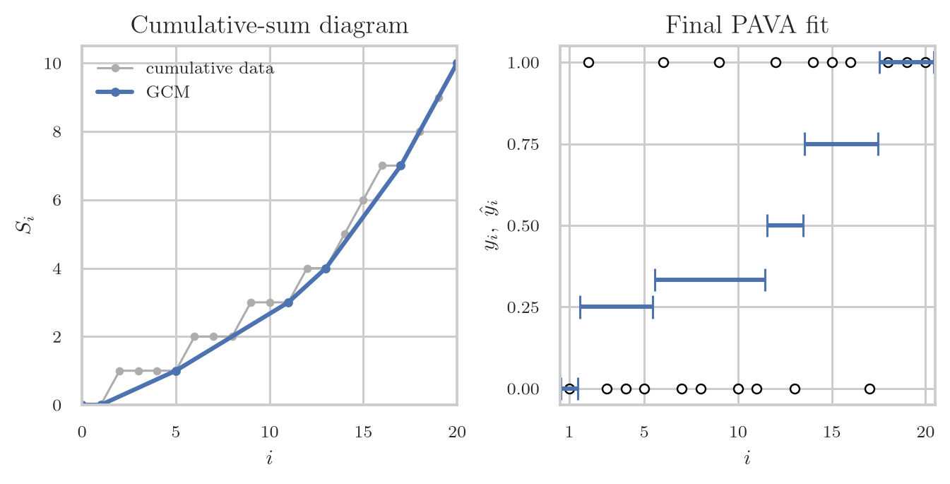
\begin{align*} \min_{\hat y: A \hat y \leq 0} \frac{1}{2} \norm{y-\hat y}^{2}. \tag{8.4.2} \end{align*}The greatest convex minorant method offers one way to find the isotonic fit. Form the cumulative sums
\begin{align*} (0,0),\ (1,S_1),\ \ldots,\ (n,S_n), \qquad S_i = \sum_{j=1}^i y_j . \end{align*}The greatest convex minorant of these points is the largest convex function on \([0,n]\) that stays below all of these points; think of a string pulled taut beneath the points, see Fig. 8.1. The isotonic fitted values \(\hat y_i\) are then the slopes of the greatest convex minorant of these cumulative points. More precisely, \(\hat y_i\) is the slope of the minorant on the segment from \(i-1\) to \(i\). We state this fact without proof; below we prove instead that PAVA solves the isotonic regression problem.
PAVA is a second method for isotonic regression. Here we
sketch its working; below we will prove that it solves the optimization problem
(8.4.2).21PAVA is supported by scikit-learn and R.
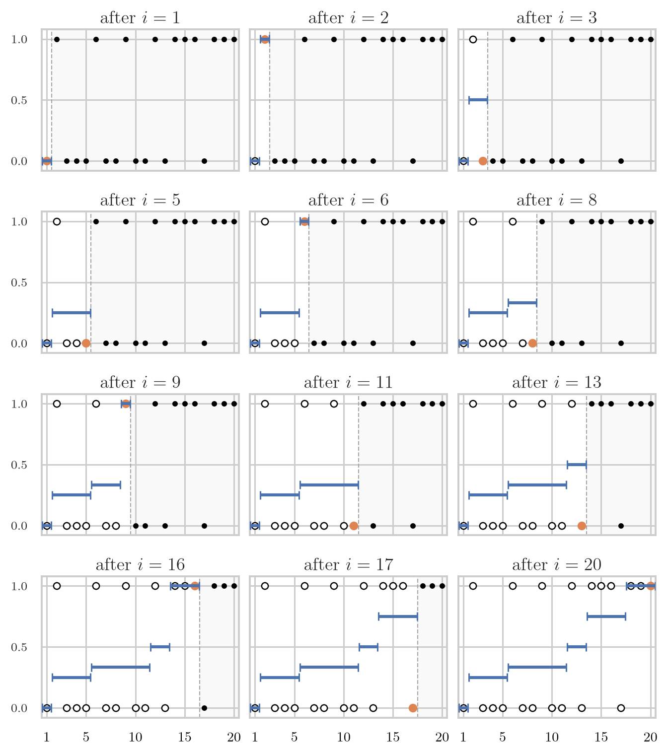
Fig. 8.2 illustrates how PAVA sweeps from left to right; Alg. 8.4.1 provides the pseudocode. It starts with one block per sorted observation, with block predictor \(\hat y_{i} = y_i\). Suppose now that two adjacent blocks \(\Lset=\set{i,\ldots,j-1}\) and \(\Rset=\set{j,\ldots,k-1}\) violate monotonicity:22Thus \(\mu_\Lset > \mu_\Rset\).
\begin{align*} \underbrace{\hat y_{i} = \cdots = \hat y_{j-1}}_{\Lset} > \underbrace{\hat y_{j} = \cdots = \hat y_{k-1}}_{\Rset}. \end{align*}Then PAVA sets
\begin{align*} \hat y_{\Mset} &= \mu_{\Mset} 1_{\Mset}, & \mu_{\Mset} &= \frac{|\Lset| \mu_{\Lset} + |\Rset|\mu_{\Rset}}{|\Mset|} = \frac{1}{|\Mset|}\sum_{l\in \Mset} y_l, & \Mset &= \Lset \cup \Rset. \tag{8.4.3} \end{align*}That is, it sets as predictor the mean of the responses on the merged set \(\Mset\). This pooled average is the barycentric mean of the two old block means, with weights given by the block sizes. 23In finding the greatest convex minorant the barycentric mean replaces the two adjacent violating slopes by the slope of the chord over their union. PAVA continues merging adjacent violators until all block averages are nondecreasing.24A careful left-to-right implementation of PAVA runs in \(O(n)\) time once the scores are sorted; the sorting step costs \(O(n\log n)\), so the full calibration procedure is typically \(O(n\log n)\).
\begin{algorithm}
\caption{Pool Adjacent Violators Algorithm}
\begin{algorithmic}
\State Start with singleton blocks $\set{1},\ldots,\set{n}$ and set $\hat y_i \gets y_i$ for all $i$.
\While{there are adjacent blocks $\Lset,\Rset$, with $\Lset$ left of $\Rset$, such that $\mu_\Lset>\mu_\Rset$}
  \State Merge the blocks $\Lset,\Rset$ into one block $\Mset = \Lset\cup\Rset$.
  \State $\mu_{\Mset}
    \gets \frac{|\Lset|\mu_\Lset+|\Rset|\mu_\Rset}{|\Mset|}$.
    \Comment{Barycentric mean}
  \State $\hat y_i \gets \mu_{\Mset}$ for every $i \in \Mset$.
\EndWhile
\Return $\hat y$
\end{algorithmic}

\end{algorithm}
Once PAVA25Or the greatest convex minorant approach. has produced the blocks with fitted values \(\hat y_i\), these blocks form bins that histogram binning can use to make the calibration function \(g\). Suppose the final blocks are \(\Iset_m=\set{s_m,\ldots,t_m}\), \(m=1,\ldots,M\), in increasing order of the scores, where \(s_m\) and \(t_m\) are the first and the last index of block \(m\). We choose bin boundaries26The PAVA fit is defined only at the observed scores in \(\Cset\); these boundaries extend it to a function on all of \([0,1]\). by setting \(b_0=0\), \(b_M=1\), and, for \(m=1,\ldots,M-1\),
\begin{align*} b_m = \frac{u_{t_m}+u_{s_{m+1}}}{2}. \end{align*}With these boundaries, the bins are as in (8.1.1) and the fitted value on block \(\Iset_m\) is its average label value, just as in (8.3.1). Hence the calibration function \(g\) can be defined by (8.3.2). Note that the scores \(u\) are not used in the isotonic regression itself, but are used to set the bin boundaries.
8.5 Cones, projections, and Moreau’s decomposition
Above we showed how PAVA works, but it remains to prove that PAVA indeed solves the isotonic regression problem (8.4.2). For this we need some concepts from convex analysis.27The geometric background used here is Salmon, Isotonic Regression. Fig. 8.3--Fig. 8.5 illustrate these definitions.
A ray is a half line emanating from the origin; in algebraic terms, if \(x\in \R^{n}\) lies in a ray, then all points \(\alpha x\) lie in the ray for \(\alpha\geq 0\). A cone is a set of rays, so a cone is closed under non-negative scaling. A convex set is such that when \(x\) and \(y\) lie in the set, the line segment \(\alpha x + (1-\alpha) y\), \(\alpha\in [0,1]\), between \(x\) and \(y\) lies in the set. A convex set is closed if its boundary belongs to it. In the sequel, a convex, closed cone \(C\) is always assumed to be nonempty. The last concept we need is the polar cone \(\polar{C}\) of \(C\) defined as
\begin{align*} \polar{C} = \set{z\in \R^{n} : \ip{z, x} \leq 0 \text{ for all } x \in C}. \end{align*}The polar cone \(\polar{C}\) is also a closed convex cone. For a nonempty closed convex cone, \(\polar{\polar{C}}=C\).28The word nonempty matters here. The empty set is also a closed convex cone, but every \(z\) satisfies the condition \(\ip{z, x} \leq 0\) for all \(x\in\varnothing\) vacuously, so \(\polar{\varnothing} = \R^{n}\). Consequently, \(\polar{\polar{\varnothing}} = \polar{(\R^{n})} = \set{0} \neq \varnothing\).
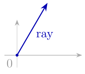
Figure 8.3: A ray starts at the origin and extends in one direction.
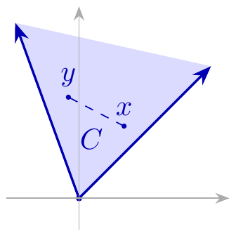
Figure 8.4: A convex cone \(C\): the segment between \(x\) and \(y\) stays in \(C\).
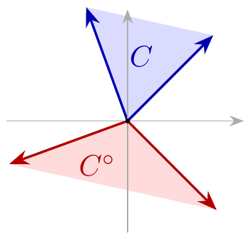
Figure 8.5: A cone \(C\) and its polar cone \(\polar{C}\).
With these definitions, we can formulate the constraint \(A \hat y \leq 0\) in (8.4.2) geometrically. Clearly the set \(K = \set{x\in \R^{n}: A x \leq 0}\) is a nonempty, closed, convex cone, so isotonic regression looks for solutions in the cone \(K\). We next study properties of this cone. First of all, we observe that the polar cone \(\polar{K}\) is well-defined.
Lemma 8.5.1.
The polar cone \(\polar{K}\) admits two further characterizations:
\begin{align*} \polar{K}_{1} &= \set{z\in \R^{n}: \lambda_i := \sum_{j=1}^i z_j \geq 0 \text{ for } i=1,\ldots,n-1, \text{ and } \lambda_n = 0}, \\ \polar{K}_{2} &= \set{A^{\top} \lambda :\lambda \in \R^{n-1}_+}. \end{align*}That is, \(\polar{K} = \polar{K}_{1} = \polar{K}_{2}.\)
Proof
To establish the equalities, we prove the cycle of inclusions \(\polar{K}_{1} \subset \polar{K}_{2} \subset \polar{K} \subset \polar{K}_{1}\).
First we show that \(\polar{K}_{1} \subset \polar{K}_{2}\). Take \(z\in \polar{K}_{1}\) and let \(\lambda_i = \sum_{j=1}^i z_j\) as in the definition of \(\polar{K}_{1}\). With the convention \(\lambda_0 = 0\), and using that \(\lambda_n = 0\) by the definition of \(\polar{K}_{1}\), we get \(z_i=\lambda_i-\lambda_{i-1}\) for \(i=1, \ldots, n\), that is, \(z=A^{\top}\lambda\). As by assumption \(\lambda_i \geq 0\) for \(i=1,\ldots,n-1\), this shows that \(z \in \polar{K}_{2}\).
Next we prove that \(\polar{K}_{2} \subset \polar{K}\). If \(z \in \polar{K}_{2}\) then \(z=A^{\top}\lambda\) with \(\lambda\geq 0\). Consequently, \(\ip{z,x} = \ip{A^{\top}\lambda, x} = \ip{\lambda, Ax} \leq 0\) because \(Ax \leq 0\) and \(\lambda\geq 0\), hence \(z\in \polar{K}\).
Finally, we show that \(\polar{K} \subset \polar{K}_{1}\). For this we need to rewrite \(\ip{z, x}\) for \(x \in K\) in a useful way.29This identity is Abel summation. It is the discrete analogue of integration by parts. Let \(\lambda_i := \sum_{j=1}^{i} z_{j}\), \(i=1, \ldots, n\), so that \(z_i = \lambda_i - \lambda_{i-1}\) if we define \(\lambda_0 = 0\). Therefore, \(\ip{z, x} = \sum_{i=1}^{n} x_i z_i = \sum_{i=1}^{n} x_i (\lambda_i - \lambda_{i-1})\). Using that \(\lambda_{0} = 0\) and relabeling,
\begin{align*} \sum_{i=1}^{n} x_{i}\lambda_{i-1} = \sum_{i=2}^{n} x_{i}\lambda_{i-1} = \sum_{i=1}^{n-1} x_{i+1}\lambda_{i}. \end{align*}With this,
\begin{align*} \ip{z, x} = \lambda_{n} x_{n} - \sum_{i=1}^{n-1} \lambda_{i}(x_{i+1}-x_{i}). \end{align*}We now use this expression to prove that \(z\in\polar{K}_{1}\) whenever \(z\in\polar{K}\). By definition of the polar cone, \(\ip{z, x}\leq 0\) for all \(x\in K\). To see that \(\lambda_n = 0\), take \(x = (1, \ldots, 1)\), which is clearly an element of \(K\). Since \(x_{i+1}-x_i=0\) in this case, \(\lambda_n x_n = \lambda_{n} \leq 0\). The constant vector \(x=(-1, \ldots, -1)\) also lies in \(K\). But then \(\ip{z, x} \leq 0\) implies that \(-\lambda_n \leq 0\). It follows that \(\lambda_n=0\). For \(\lambda_i\), \(i=1,\ldots, n-1\), take the vector \(x=(0, \ldots, 0, 1, \ldots, 1)\) with \(x_k=0\) for \(k\leq i\) and \(x_k=1\) for \(k>i\). This vector belongs to \(K\), and
\begin{align*} \ip{z, x} = \sum_{k=i+1}^n z_k = \lambda_n-\lambda_i = -\lambda_i. \end{align*}Since \(\ip{z,x}\leq 0\), this implies that \(\lambda_i\geq 0\). Thus \(\lambda_i\geq 0\) for \(i=1,\ldots,n-1\) and \(\lambda_n=0\), so \(z\in\polar{K}_{1}\). This proves \(\polar{K}\subset\polar{K}_{1}\) and completes the proof.
Moreau's decomposition theorem is the key building block for the proof of PAVA. It relies on the projection theorem, which we prove first.
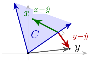
Figure 8.6: The projection theorem.
Given a nonempty closed convex set \(C\subseteq\R^{n}\), the projection of \(y\in\R^{n}\) onto \(C\) is defined as \(P_C(y) = \argmin_{x \in C} \norm{y-x}\).
Theorem 8.5.2.
The projection theorem, see Fig. 8.6. Let \(C\) be a nonempty, convex, closed set in \(\R^{n}\). Then,
- The projection is well defined: for every \(y\in\R^{n}\), the minimum defining the projection \(P_C(y)\) exists and is unique.
- A point \(\hat y \in C\) is the projection \(P_C(y)\) of a point \(y\) iff \(\ip{y-\hat y, x-\hat y}\leq 0\) for all \(x\in C\).
Proof
For 1, since \(C\) is nonempty, pick \(z\in C\). The intersection of \(C\) with the closed ball \(D\) with center \(y\) and radius \(\norm{z-y}\), i.e., \(D\cap C\), is compact. Since the function \(x\to\norm{x-y}\) is continuous, it attains its minimum at some point \(\hat y\) in \(D\cap C\). Any point in \(C\setminus D\) has distance greater than \(\norm{z-y}\) to \(y\), hence \(C\setminus D\) cannot contain a minimizer. Therefore \(\hat y\) minimizes the distance to \(y\) over all of \(C\).
If \(y \in C\), then \(y = P_C(y) = \hat y\): the minimal distance is \(0\), and it is attained at \(y\) only. Moreover, \(\ip{y - \hat y, x - \hat y} = 0\) for all \(x\in C\), so the inequality in 2 holds trivially. Assume therefore that \(y \notin C\), so that \(\norm{y - \hat y} > 0\).
Consider now an open ball \(B\) with center \(y\) and radius \(\norm{y-\hat y}\), hence \(\hat y \not \in B\), but \(\hat y\) is an element of the closure \(\overline B\) of \(B\). As \(\hat y\in C\) is a point closest to \(y\) in \(C\), \(B\cap C = \varnothing\). However, \(\hat y\in C\cap\overline B\), see Fig. 8.7.
Moreover, as \(C\) and \(B\) are both convex, by the separating hyperplane theorem there exists a hyperplane that separates \(B\) and \(C\). This hyperplane must pass through \(\hat y\), and as \(B\) is a ball, it is tangent to \(B\) at \(\hat y\). Consequently, the vector \(y-\hat y\) is normal to this hyperplane. As \(x\in C\) and \(y\in B\) lie on opposite sides of this plane, \(\ip{y-\hat y, x-\hat y} \leq 0\).
We can now also settle uniqueness. Any minimizer lies in \(C\cap\overline B\). Since \(C\) and \(\overline B\) lie at opposite sides of the hyperplane, \(C\cap\overline B\) is part of the hyperplane itself, and the hyperplane, being tangent to the ball, meets \(\overline B\) only at \(\hat y\). Hence \(C\cap\overline B=\set{\hat y}\): the minimizer is unique.
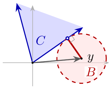
Figure 8.7: The open ball \(B\) centered at \(y\) touches the cone \(C\) at the small open circle indicating \(\hat y\). Since \(B\) is open, it is disjoint from \(C\).
Finally, suppose that \(p\in C\) is such that \(\ip{y -p, x - p} \leq 0\) for all \(x \in C\). Then
\begin{align*} \norm{y-x}^{2} = \norm{y-p + p - x}^{2} = \norm{y-p}^{2} + \norm{p-x}^{2} + 2\ip{y-p, p-x}. \end{align*}As \(\norm{p-x} \geq 0\) and \(\ip{y-p, p-x}\ge 0\) by assumption, \(\norm{x-y} \geq \norm{y-p}\) for all \(x\in C\). Thus \(p\) is the point closest in \(C\) to \(y\), and therefore \(p=\hat y = P_C(y)\).
The projection theorem is the main tool for proving the next theorem.
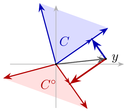
Figure 8.8: Projection arrows in Moreau’s decomposition: from \(y\) to \(\hat y=P_C(y)\) and from \(y\) to \(\polar{y}=P_{\polar{C}}(y) = y - \hat y\).
Theorem 8.5.3.
Moreau’s decomposition theorem, see Fig. 8.8. Let \(C\) be a nonempty, closed, convex cone with polar cone \(\polar{C}\). Then,
- For every \(y\in\R^{n}\), there exist unique projections \(\hat y = P_C(y)\) on \(C\) and \(\polar{y} = P_{\polar{C}}(y)\) on the polar cone \(\polar{C}\), such that \(y=\hat y + \polar{y}\) and \(\ip{\hat y, \polar{y}} = 0\).
- Moreover, if \(y=r+s\) with \(r\in C\), \(s\in \polar{C}\) and \(\ip{r,s}=0\), then \(r=P_C(y)\) and \(s=P_{\polar{C}}(y)\).
Proof
By the projection theorem, \(\hat y=P_C(y)\) exists and is unique. We first prove that \(y-\hat y \in \polar{C}\). By the projection theorem, \(\ip{y-\hat y, z - \hat y} \leq 0\) for all \(z\in C\). As \(C\) is a cone, \(0\in C\) and \(2\hat y\in C\), therefore
\begin{align*} 0 &\geq \ip{y-\hat y, 0 - \hat y} = - \ip{y - \hat y, \hat y}, \\ 0 &\geq \ip{y-\hat y, 2\hat y - \hat y} = \ip{y - \hat y, \hat y}. \end{align*}It follows that \(\ip{y - \hat y, \hat y} = 0\). Now take any \(z\in C\). Then
\begin{align*} \ip{y - \hat y, z} = \ip{y-\hat y, z - \hat y} + \ip{y-\hat y, \hat y} \leq 0. \end{align*}Consequently, \(y-\hat y \in \polar{C}\).
Next we prove that \(y-\hat y=P_{\polar{C}}(y)\). Let \(p=y-\hat y\). For any \(x\in \polar{C}\),
\begin{align*} \ip{y-p, x-p} &= \ip{\hat y, x-(y-\hat y)}\\ &= \ip{\hat y, x} - \ip{\hat y, y-\hat y}\\ &\leq 0. \end{align*}Here \(\ip{\hat y,x}\leq 0\) because \(\hat y\in C\) and \(x\in\polar{C}\), while \(\ip{\hat y,y-\hat y}=0\) by the previous paragraph. The projection theorem gives \(p=P_{\polar{C}}(y)\). Hence, with \(\polar{y}=p\),
\begin{align*} y = \hat y + \polar{y},\qquad \hat y = P_C(y),\qquad \polar{y}=P_{\polar{C}}(y),\qquad \ip{\hat y,\polar{y}}=0. \end{align*}Finally, suppose that \(y=r+s\) with \(r\in C\), \(s\in\polar{C}\) and \(\ip{r,s}=0\). For any \(x\in C\),
\begin{align*} \ip{y-r,x-r} = \ip{s,x-r} = \ip{s,x} - \ip{s,r} \leq 0. \end{align*}Thus \(r=P_C(y)\). Similarly, for any \(x\in\polar{C}\),
\begin{align*} \ip{y-s,x-s} = \ip{r,x-s} = \ip{r,x} - \ip{r,s} \leq 0, \end{align*}so \(s=P_{\polar{C}}(y)\).
8.6 Why PAVA works
Moreau’s theorem allows us to show that PAVA produces the projection \(\hat y = P_K(y)\) of the responses \(y\) on the cone \(K=\set{x\in \R^{n}: A x \leq 0}\). As this projection is the solution of the isotonic regression problem, it then follows that PAVA works. The procedure of the proof is to focus on consecutive blocks and repair any violations of the constraint \(A x\leq 0\) one by one until no violations remain.
We need one further notational device. When \(\Iset\) is a set of consecutive indices, then we write \(y_\Iset\) for the restriction of \(y\) to \(\Iset\), and \(1_\Iset\) for the vector indexed by \(\Iset\) whose components are all \(1\). Furthermore, \(K_\Iset=\set{x \in \R^{|\Iset|} : A x \leq 0}\), where \(A\) is the matrix of (8.4.1), now of size \((|\Iset|-1)\times|\Iset|\); in words, \(K_\Iset\) consists of the nondecreasing vectors indexed by \(\Iset\).
Throughout its sweep, PAVA maintains a partition of \(\set{1,\ldots,n}\) into blocks of consecutive indices. On each block \(\Iset = \set{a, \ldots, b}\) let
\begin{align*} \hat y_\Iset &= \mu_{\Iset} 1_{\Iset}, & \mu_\Iset &= \frac{1}{|\Iset|} \sum_{l \in \Iset} y_{l}. \tag{8.6.1} \end{align*}Suppose that on each block the residual \(\rscr_{\Iset}\) with components \(\rscr_{\Iset,l}=y_l-\mu_\Iset\) satisfies
\begin{align*} \sum_{l=a}^{m} \rscr_{\Iset,l}&\geq 0 \quad m \in \Iset, & \sum_{l=a}^{b} \rscr_{\Iset,l} &=0. \end{align*}In words, as we move through the block from left to right, the accumulated excess over the block average never becomes negative, and it is zero at the right end of the block. By the first polar-cone characterization in Lem. 8.5.1, applied with \(n\) replaced by \(|\Iset|\) it follows that \(\rscr_\Iset\in\polar K_\Iset\).
Lemma 8.6.1.
If \(\hat y_{\Iset}\) is as in (8.6.1) and the residual \(\rscr_\Iset = y_{\Iset}-\hat y_{\Iset} \in \polar{K}_{\Iset}\), then \(\ip{\rscr_\Iset, \hat y_\Iset} = 0\), \(\hat y_\Iset = P_{K_\Iset}(y_\Iset)\), and \(\rscr_\Iset = P_{\polar{K}_{\Iset}}(y_\Iset)\).
Proof
Since \(\hat y_\Iset\) has constant components \(\mu_\Iset\), \(A \hat y_\Iset = \mu_{\Iset} A 1_{\Iset} = 0\). Hence, \(\hat y_\Iset \in K_\Iset\). Second, the residual \(\rscr_\Iset = y_\Iset - \hat y_\Iset\) is orthogonal to \(\hat y_\Iset\):
\begin{align*} \ip{\rscr_{\Iset}, \hat y_{\Iset}} = \ip{y_{\Iset}, \hat y_{\Iset}} -\ip{\hat y_{\Iset}, \hat y_{\Iset}} = \mu_{\Iset} \ip{y_{\Iset}, 1_{\Iset}} -\mu_{\Iset}^{2}\ip{1_{\Iset}, 1_{\Iset}} = 0, \tag{8.6.2} \end{align*}because \(\ip{y_{\Iset}, 1_{\Iset}} = \mu_\Iset |\Iset|\) and \(\ip{1_{\Iset}, 1_{\Iset}} = |\Iset|\). Third, by assumption \(\rscr_\Iset\in\polar K_\Iset\). Thus we have vectors \(\hat y_\Iset \in K_\Iset\) and \(\rscr_\Iset \in \polar{K}_{\Iset}\) with \(y_\Iset = \hat y_\Iset + \rscr_\Iset\) and \(\ip{\rscr_\Iset, \hat y_\Iset} = 0\), so Moreau’s theorem implies that \(\hat y_\Iset = P_{K_\Iset}(y_\Iset)\).
We show next that pooling two adjacent violating blocks with PAVA establishes that the residual on the merged set is again in a suitable polar cone.
Lemma 8.6.2.
Assume that \(\rscr_{\Lset} \in \polar{K}_{\Lset}\) and \(\rscr_{\Rset} \in \polar{K}_{\Rset}\). If \(\Lset\) and \(\Rset\) are adjacent violators, then \(\rscr_{\Mset} = y_{\Mset} - \hat y_{\Mset} \in\polar{K}_{\Mset}\), where \(\Mset\) and \(\hat y_\Mset\) are given by (8.4.3).
Proof
First, \(\hat y_{\Mset}\), being constant, lies in the cone \(K_{\Lset \cup \Rset}\). To see that the pooled residual \(\rscr_\Mset \in \polar{K}_{\Mset}\), we reason as follows. As \(\mu_{\Lset} > \mu_\Mset > \mu_\Rset\), it must be that on \(\Lset\), each residual \(y_{l} - \mu_{\Mset}\) is larger than the old residual \(y_{l} - \mu_\Lset\), so all accumulated sums inside \(\Lset\) increase; in particular, the accumulated excess at the right end of \(\Lset\) rises from \(0\) to \(|\Lset|(\mu_\Lset-\mu_{\Mset}) > 0\). On \(\Rset\), each new residual is the old residual minus \(\mu_{\Mset} - \mu_\Rset\), so after \(m\) elements of \(\Rset\) the accumulated excess has dropped by \(m(\mu_{\Mset}-\mu_\Rset)\), which is at most \(|\Rset|(\mu_{\Mset} - \mu_\Rset)\). The definition of the pooled mean gives
\begin{align*} |\Lset|(\mu_\Lset-\mu_{\Mset}) =|\Rset|(\mu_{\Mset} - \mu_\Rset), \end{align*}so the drop on \(\Rset\) never exceeds the surplus gained at the right end of \(\Lset\). Therefore the accumulated sum stays positive on the merged block, except at the right end: there the surplus and the deficit cancel exactly, so the total sum is \(0\).
It is interesting to see why we should not merge when \(\mu_\Lset < \mu_\Rset\). In this case \(\mu_\Mset > \mu_\Lset\), so the accumulated sum at the right end of \(\Lset\) drops from \(0\) to \(|\Lset|(\mu_\Lset - \mu_\Mset) < 0\): the pooled residual violates the partial-sum condition, that is, \(\rscr_\Mset \not\in \polar{K}_{\Mset}\).
By combining Lem. 8.6.1 with Lem. 8.6.2, we obtain the following.
Corollary 8.6.3.
Under the conditions of Lem. 8.6.2,
\begin{align*} \hat y_\Mset &= P_{K_\Mset}(y_\Mset), & \rscr_\Mset &= P_{\polar{K}_{\Mset}}(y_\Mset), & \ip{\rscr_\Mset,\hat y_\Mset} &= 0. \end{align*}PAVA starts with \(n\) singleton blocks \(\Bset_i=\set{i}\). On each block, the residual is zero and hence belongs to \(\polar{K}_{\Bset_i}\). Each pooling step reduces the number of blocks by one, and by Lem. 8.6.2, it maintains the loop invariant that on a merged block \(\rscr_\Mset\in\polar{K_\Mset}\) and \(\hat y_\Mset=P_{K_\Mset}(y_\Mset)\). Thus PAVA terminates after at most \(n-1\) pooling steps.
At termination, the block means are nondecreasing, so \(\hat y\in K\). Every partial sum of the full residual \(\rscr=y-\hat y\) is nonnegative: completed blocks contribute zero, and the remaining partial block contributes a nonnegative sum. The total sum is zero. By the polar-cone characterization, \(\rscr\in\polar{K}\). Summing the blockwise orthogonality identities of (8.6.2) gives \(\ip{\rscr,\hat y}=0\). Moreau’s theorem therefore yields \(\hat y=P_K(y)\). Consequently,
Theorem 8.6.4.
PAVA computes the solution of the isotonic regression problem.
The KKT conditions connect the geometric projection proof to constrained optimization. The projection of \(y\) on the cone \(K\) is the constrained optimization problem
\begin{align*} \min_{x \in K} \frac{1}{2} \norm{x - y}^{2}. \end{align*}We take this problem as the primal problem and derive its dual. This shows that the polar-cone residual in Moreau’s theorem is the dual optimizer, and that orthogonality becomes complementary slackness. The Lagrangian is
\begin{align*} \mathscr{L}(x, \lambda) = \frac{1}{2} \norm{x - y}^{2} + \ip{\lambda, Ax}, \quad \lambda \in \R^{n-1}_{+}. \end{align*}Setting the derivative of \(\mathscr{L}\) with respect to \(x\) to \(0\) and solving for \(x\) gives \(x=y - A^{\top} \lambda\). Write this solution as \(\hat y = y - A^{\top} \lambda\). Inserting this in the Lagrangian gives the dual problem
\begin{align*} \max_{\lambda \geq 0} \set{- \frac{1}{2} \norm{A^{\top} \lambda}^{2} + \ip{\lambda, Ay}}. \end{align*}Now define \(\rscr=A^{\top} \lambda\), so that the dual objective becomes \(-\frac{1}{2} \norm{\rscr}^{2} + \ip{\rscr, y}\) with \(\rscr\in \polar{K}\), by the second characterization of the polar cone in Lem. 8.5.1. Completing the square gives
\begin{align*} -\frac{1}{2} \norm{\rscr}^{2} + \ip{\rscr, y} = -\frac{1}{2}\norm{y-\rscr}^{2} + \frac{1}{2} \norm{y}^{2}. \end{align*}Since the last term is a constant, maximizing the dual is the same as
\begin{align*} \min_{\rscr\in \polar{K}} \frac{1}{2}\norm{y-\rscr}^{2}. \end{align*}This is precisely the projection of \(y\) on \(\polar{K}\). The projections of \(y\) on \(K\) and on \(\polar{K}\) solve the primal and the dual problem simultaneously.
The projection theorem gives unique solutions on \(K\) and on its polar cone \(\polar{K}\). As \(\hat y = P_K(y) \in K\), \(\hat y\) satisfies primal feasibility, likewise, by Lem. 8.6.2, \(\rscr = y - \hat y \in \polar{K}\), hence \(\rscr\) satisfies dual feasibility. By Moreau’s theorem, \(0=\ip{\rscr, \hat y} = \ip{A^{\top} \lambda, \hat y} = \ip{\lambda, A\hat y}\). Since \(\lambda_i \geq 0\) and \((A\hat y)_i \leq 0\), every term of this sum is nonpositive, so each must be zero: \(\lambda_i (A\hat y)_i = 0\) for all \(i\), which is complementary slackness. Finally, stationarity of the Lagrangian at the optimum is expressed by
\begin{align*} \nabla_x\mathscr{L}(\hat y,\lambda) = \hat y-y+A^\top\lambda=0. \end{align*}8.7 Exercises
Conceptual 1.
A random forest ranks the OSM edges of the walking-route planner from good to bad. Why is this ranking not enough for the routing step, and what does the calibration map \(g\) of this chapter add to it?
Solution
A routing algorithm needs a cost per edge, because it adds the costs along a route and compares the sums. A ranking only orders the edges: it does not say how much worse one edge is than the next, so differences in rank cannot be added. The map \(g\) turns the score of the forest into a probability, a number on a scale on which such differences do mean something, and that probability becomes the edge cost.
Conceptual 2.
Sigmoid scaling, histogram binning, and isotonic regression all choose a calibration function \(g\) by minimizing an empirical risk on the calibration list \(\Cset\). For each method, which loss function does it minimize, and over which class of calibration functions does it minimize? Relate each loss to maximum likelihood under a model for the labels \(Y_i\).
Solution
The three methods differ in the loss and in the class of functions:
| Method | Loss | Calibration functions \(g\) |
|---|---|---|
| Sigmoid scaling | cross-entropy | \(g_{a,b}(u)=\sigma(au+b)\) |
| Histogram binning | squared error (Brier) | constant on each of the fixed bins |
| Isotonic regression | squared error (Brier) | all nondecreasing functions |
The losses are maximum likelihood in disguise. If \(Y_i\sim\Bern{\hat p_i}\), then maximum likelihood gives the cross-entropy loss, as in (5.1.5). If, as an approximation, \(Y_i\sim\Norm{\hat p_i,v}\) with common variance \(v\), then maximum likelihood gives squared error, hence the Brier score.
The methods differ in how \(\hat p_i\) depends on the score. In sigmoid scaling, \(\hat p_i=g_{a,b}(u_i)=\sigma(au_i+b)\) for the two-parameter family \(g_{a,b}\). In histogram binning and isotonic regression, \(\hat p_i=g(u_i)\), where \(g\) is the calibration function that we still have to find. Histogram binning minimizes squared error after the bins are fixed. Isotonic regression minimizes squared error under the condition that \(g\) must be nondecreasing.
Technical 3.
Use the three bins \(B_1=[0,0.3)\), \(B_2=[0.3,0.6)\), and \(B_3=[0.6,1]\), and the calibration data
| Score \(u_i\) | Label \(y_i\) |
|---|---|
| 0.10 | 0 |
| 0.20 | 0 |
| 0.30 | 1 |
| 0.50 | 0 |
| 0.60 | 1 |
| 0.80 | 1 |
Make a reliability curve for the uncalibrated scores in this data.
Solution
The average scores and observed positive fractions in the three bins are
| Bin | Average score \(\bar u_m\) | Positive fraction \(\hat p_m\) |
|---|---|---|
| \(B_1\) | 0.15 | 0 |
| \(B_2\) | 0.40 | 0.5 |
| \(B_3\) | 0.70 | 1 |
Plot the points \((0.15,0)\), \((0.40,0.5)\), and \((0.70,1)\), with the diagonal \(\hat p=\bar u\) as a reference.
Conceptual 4.
PAVA merges two adjacent blocks when their means violate monotonicity. Why does the merged block take the size-weighted, or barycentric, mean of the two block means? Why is the ordinary mean of the two block means not always right?
Solution
The merged block gives every observation in the union the same fitted value. Under squared loss, the best such value is the mean of all labels in the combined block. If the old blocks have sizes \(|\Lset|\) and \(|\Rset|\), and means \(\mu_\Lset\) and \(\mu_\Rset\), this value is \[ \frac{|\Lset|\mu_\Lset+|\Rset|\mu_\Rset}{|\Lset|+|\Rset|}. \] The unweighted mean gives the same answer only when the two blocks have equal size; otherwise it does not preserve the mean of all labels in the merged block.
Algorithmical 5.
The labels \((0,1,0,0,1,0)\) are ordered by increasing score. Carry out PAVA graphically: draw the singleton blocks and their means, show each merge of adjacent blocks whose means decrease, and give the final fitted values.
Solution
Start with the six singleton blocks \[ 0\mid 1\mid 0\mid 0\mid 1\mid 0. \] Merge the second and third blocks, then merge that block with the fourth: \[ 0\mid [1,0]_{1/2}\mid 0\mid 1\mid 0 \quad\longrightarrow\quad 0\mid [1,0,0]_{1/3}\mid 1\mid 0. \] Finally merge the last two blocks: \[ 0\mid [1,0,0]_{1/3}\mid [1,0]_{1/2}. \] The block means are now nondecreasing. The fitted values are \((0,\frac13,\frac13,\frac13,\frac12,\frac12)\).
Algorithmical 6.
Let \(C=\{x\in\R^3:x_1\leq x_2\leq x_3\}\), \(y=(0,2,1)\), and \(\hat y=(0,\frac32,\frac32)\). Verify using Moreau’s theorem that \(\hat y=P_C(y)\).
Solution
First, \(\hat y\in C\). The residual is \(r=y-\hat y=(0,\frac12,-\frac12)\). For any \(x\in C\), \(\ip{r,x}=\frac12(x_2-x_3)\leq 0\), so \(r\in\polar{C}\). Also, \[ \ip{\hat y,r}=0\cdot0+\frac32\cdot\frac12 +\frac32\cdot\rb{-\frac12}=0. \] Thus \(y=\hat y+r\) is a decomposition into orthogonal vectors in \(C\) and \(\polar{C}\). Moreau’s theorem gives \(\hat y=P_C(y)\).
Technical 7.
Prove Moreau’s decomposition theorem. That is, for a nonempty, closed, convex cone \(C\), prove that every \(y\) has a unique decomposition \[ y=P_C(y)+P_{\polar{C}}(y), \qquad \ip{P_C(y),P_{\polar{C}}(y)}=0. \] Also prove the converse: if \(y=r+s\), where \(r\in C\), \(s\in\polar{C}\), and \(\ip{r,s}=0\), then \(r=P_C(y)\) and \(s=P_{\polar{C}}(y)\).
Solution
See the proof in the book.